FSharp.Azure.Quantum
1.6.2
dotnet add package FSharp.Azure.Quantum --version 1.6.2
NuGet\Install-Package FSharp.Azure.Quantum -Version 1.6.2
<PackageReference Include="FSharp.Azure.Quantum" Version="1.6.2" />
<PackageVersion Include="FSharp.Azure.Quantum" Version="1.6.2" />
<PackageReference Include="FSharp.Azure.Quantum" />
paket add FSharp.Azure.Quantum --version 1.6.2
#r "nuget: FSharp.Azure.Quantum, 1.6.2"
#:package FSharp.Azure.Quantum@1.6.2
#addin nuget:?package=FSharp.Azure.Quantum&version=1.6.2
#tool nuget:?package=FSharp.Azure.Quantum&version=1.6.2
FSharp.Azure.Quantum
Quantum-First F# Library - Solve combinatorial optimization problems using quantum algorithms (QAOA - Quantum Approximate Optimization Algorithm), on a local simulator by default or on cloud backends when you pass one.


flowchart TD

    %% Top layer
    A[.NET API High-level algorithms familiar to normal developers]

    %% Quantum algorithms
    B[Quantum Algorithms,
       Ph.D stuff]

    %% Backend interfaces
    C[Backend Interfaces: IQuantumBackend]

    %% Quantum Gate Backends
    D[Quantum Gate Backends:
        LocalSimulator: Ph.D stuff,
        Azure Quantum as a service]


    %% Topological Backends
    E[Topological Backend simulator,
       more Ph.D stuff]

    %% Flow
    A --> B --> C
    C --> D
    C --> E
Table of Contents
- Status
- Quick Start
- Problem Builders
- Advanced Quantum Builders
- Quantum Machine Learning (QML)
- Business Problem Builders
- HybridSolver
- Architecture
- OpenQASM 2.0 Support
- Error Mitigation
- QAOA Algorithm Internals
- Documentation
- Problem Size Guidelines
- Design Philosophy
- Quantum Algorithms
- Topological Quantum Computing
- Contributing
- License
- Support
Status
Architecture: Quantum-First Hybrid Library - Quantum algorithms as primary solvers, with opt-in classical routing (via HybridSolver / QuantumAdvisor) for small problems where quantum offers no advantage. Quantum solvers never fall back to classical silently — see Design Philosophy.
Current Version: 1.6.2 (core) / 0.6.2 (Topological and Braket plugins) — D-Wave Support + Quantum Machine Learning + Business Builders + compilation/hardware tooling (QIR, resource estimation, qubit routing, noise-aware routing)
Current Features:
- Multiple Backends: LocalBackend (simulation), NoisyLocalBackend (density-matrix noise), Azure Quantum (IonQ, Rigetti, Quantinuum, Atom Computing, IQM), D-Wave quantum annealers (1200-5640 qubits), AWS Braket (separate plugin)
- Cloud execution: the QAOA solvers, UCCSD-VQE and QPE chemistry, Grover and its builders, amplitude amplification, QFT, QPE, Shor, HHL, quantum arithmetic, ADAPT-VQE/ADAPT-QAOA, QML, quantum Monte Carlo pricing and risk,
Primitivesand the textbook protocols (Bell, teleportation, superdense coding, Deutsch-Jozsa, Bernstein-Vazirani, Simon, BB84, E91, bit- and phase-flip codes) build complete circuits and submit them as whole-circuit jobs, transpiled to each provider's native gates. Every job is billed; aJobBudgetcaps how many a run may submit - Topological Quantum Computing: Anyon braiding simulator (Ising, Fibonacci & SU(2)_k anyons) with error correction (toric code, surface codes, anyonic charge correction) - Microsoft Majorana architecture
- Quantum Machine Learning: VQC, Quantum Kernel SVM, Feature Maps, Variational Forms, AutoML
- Business Problem Builders: Social Network Analysis, Constraint Scheduling, AutoML, Anomaly Detection, Binary Classification, Predictive Modeling, Similarity Search
- OpenQASM 2.0: Import/export compatibility with IBM Qiskit, Amazon Braket, Google Cirq
- QAOA Implementation: Quantum Approximate Optimization Algorithm with advanced parameter optimization
- 7 Quantum Optimization Builders: Graph Coloring, MaxCut, Knapsack, TSP, Portfolio, Network Flow, Task Scheduling
- 6 Advanced Builders: Quantum Arithmetic, Cryptographic Analysis (Shor's), Phase Estimation (QFT/QPE-based); Tree Search, Constraint Solver, Pattern Matcher (Grover-based)
- VQE Implementation: Variational Quantum Eigensolver for molecular ground state energies (quantum chemistry), plus ground-state energies by quantum phase estimation (
GroundStateMethod.QPE) - Error Mitigation: ZNE (typically 30-50% error reduction), PEC (typically 50-80% error reduction), REM (typically 50-90% readout error reduction), strategy selection. The percentages are typical ranges reported in the literature, not guarantees.
- F# Computation Expressions: Idiomatic, type-safe problem specification with builders
- C# Interop: Fluent API extensions for C# developers
- Circuit Building: Low-level quantum circuit construction and optimization possible
Quick Start
Installation
dotnet add package FSharp.Azure.Quantum
In an F# script (.fsx), reference the package instead; dotnet add package does not reach scripts:
#r "nuget: FSharp.Azure.Quantum"
The examples do this already:
download the examples folder and run any script with dotnet fsi <script>.fsx, with no build of this
repository needed. See Running Examples.
F# Computation Expressions
open System.Threading
open FSharp.Azure.Quantum
open FSharp.Azure.Quantum.GraphColoring

// Graph Coloring: Register Allocation
let problem = graphColoring {
    node "R1" ["R2"; "R3"]
    node "R2" ["R1"; "R4"]
    node "R3" ["R1"; "R4"]
    node "R4" ["R2"; "R3"]
    colors ["EAX"; "EBX"; "ECX"; "EDX"]
}

// Solve using quantum optimization (QAOA)
task {
    match! GraphColoring.solveAsync problem 4 None CancellationToken.None with
    | Ok solution ->
        printfn "Colors used: %d" solution.ColorsUsed
        solution.Assignments
        |> Map.iter (fun node color -> printfn "%s → %s" node color)
    | Error err ->
        printfn "Error: %s" err.Message
}
Samples are task blocks: await them in an application, or end a script with |> Async.AwaitTask |> Async.RunSynchronously.
C# Fluent API
using System.Threading;
using FSharp.Azure.Quantum;
using static FSharp.Azure.Quantum.CSharpBuilders;

// MaxCut: Circuit Partitioning
var vertices = new[] { "A", "B", "C", "D" };
var edges = new[] {
    (source: "A", target: "B", weight: 1.0),
    (source: "B", target: "C", weight: 2.0),
    (source: "C", target: "D", weight: 1.0),
    (source: "D", target: "A", weight: 1.0)
};

var problem = MaxCutProblem(vertices, edges);
var result = await MaxCut.solveAsync(problem, null, CancellationToken.None);

if (result.IsOk) {
    var solution = result.ResultValue;
    Console.WriteLine($"Cut Value: {solution.CutValue}");
    Console.WriteLine($"Partition S: {string.Join(", ", solution.PartitionS)}");
    Console.WriteLine($"Partition T: {string.Join(", ", solution.PartitionT)}");
}
What happens:
- Computation expression builds graph coloring problem
GraphColoring.solveAsynccallsQuantumGraphColoringSolverinternally- QAOA quantum algorithm encodes problem as QUBO (Quadratic Unconstrained Binary Optimization)
- LocalBackend simulates quantum circuit (memory-derived width)
- Returns color assignments with validation
Problem Builders
Optimization Builders using QAOA:
Graph Coloring
Use Case: Register allocation, frequency assignment, exam scheduling
open System.Threading
open FSharp.Azure.Quantum
open FSharp.Azure.Quantum.GraphColoring

let problem = graphColoring {
    node "Task1" ["Task2"; "Task3"]
    node "Task2" ["Task1"; "Task4"]
    node "Task3" ["Task1"; "Task4"]
    node "Task4" ["Task2"; "Task3"]
    colors ["Slot A"; "Slot B"; "Slot C"]
    objective MinimizeColors
}

task {
    match! GraphColoring.solveAsync problem 3 None CancellationToken.None with
    | Ok solution ->
        printfn "Valid coloring: %b" solution.IsValid
        printfn "Colors used: %d/%d" solution.ColorsUsed 3
        printfn "Conflicts: %d" solution.ConflictCount
    | Error err -> printfn "Error: %s" err.Message
}
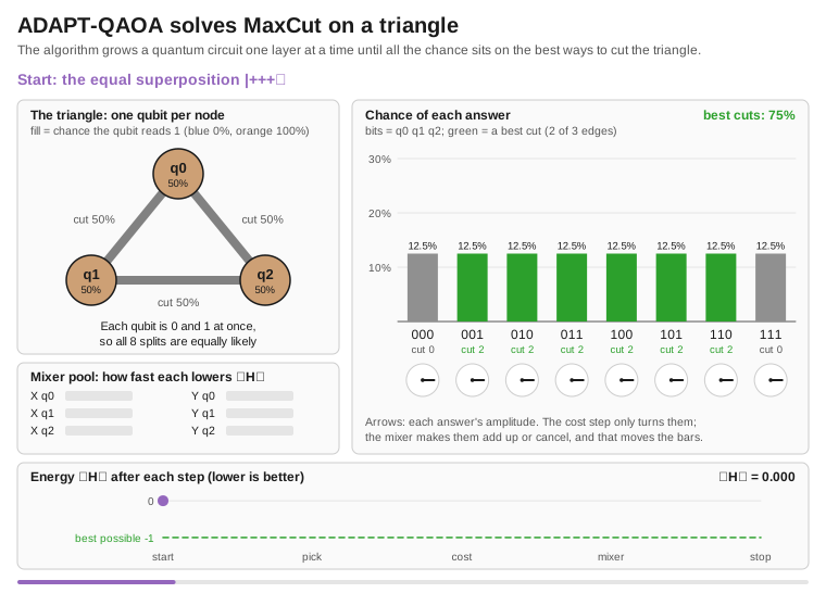
MaxCut
Use Case: Circuit design, community detection, load balancing
let vertices = ["A"; "B"; "C"; "D"]
let edges = [
    ("A", "B", 1.0)
    ("B", "C", 2.0)
    ("C", "D", 1.0)
    ("D", "A", 1.0)
]

let problem = MaxCut.createProblem vertices edges

task {
    match! MaxCut.solveAsync problem None CancellationToken.None with
    | Ok solution ->
        printfn "Partition S: %A" solution.PartitionS
        printfn "Partition T: %A" solution.PartitionT
        printfn "Cut value: %.2f" solution.CutValue
    | Error err -> printfn "Error: %s" err.Message
}
Knapsack (0/1)
Use Case: Resource allocation, portfolio selection, cargo loading
let items = [
    ("laptop", 3.0, 1000.0)   // (id, weight, value)
    ("phone", 0.5, 500.0)
    ("tablet", 1.5, 700.0)
    ("monitor", 2.0, 600.0)
]

let problem = Knapsack.createProblem items 5.0  // capacity = 5.0

task {
    match! Knapsack.solveAsync problem None CancellationToken.None with
    | Ok solution ->
        printfn "Total value: $%.2f" solution.TotalValue
        printfn "Total weight: %.2f/%.2f" solution.TotalWeight problem.Capacity
        printfn "Items: %A" (solution.SelectedItems |> List.map (fun i -> i.Id))
    | Error err -> printfn "Error: %s" err.Message
}
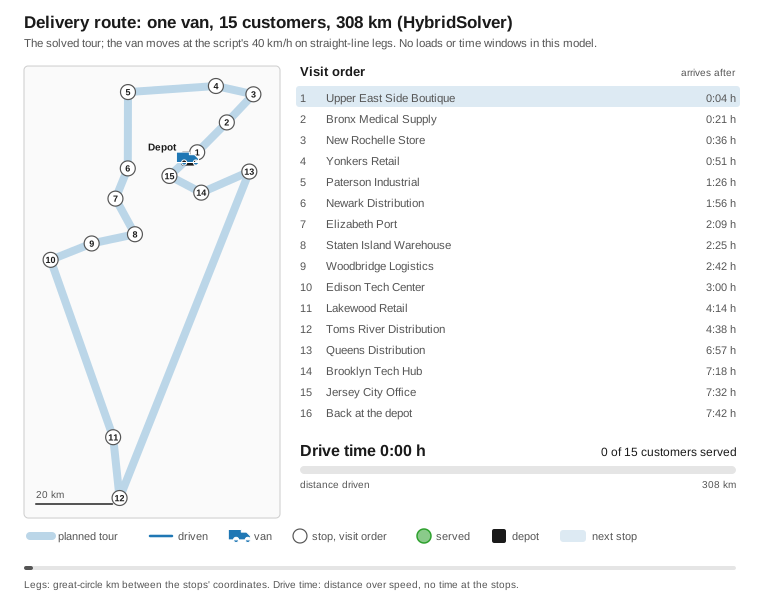
Traveling Salesperson Problem (TSP)
Use Case: Route optimization, delivery planning, logistics
let cities = [
    ("Seattle", 0.0, 0.0)
    ("Portland", 1.0, 0.5)
    ("San Francisco", 2.0, 1.5)
    ("Los Angeles", 3.0, 3.0)
]

let problem = TSP.createProblem cities

task {
    match! TSP.solveAsync problem None CancellationToken.None with
    | Ok tour ->
        printfn "Route: %s" (String.concat " → " tour.Cities)
        printfn "Total distance: %.2f" tour.TotalDistance
    | Error err -> printfn "Error: %s" err.Message
}
Four cities are 16 qubits (cities²). The default configuration optimises two QAOA layers, which takes a minute or two on the local simulator. A measurement counts as a route only when it places every city in exactly one time slot; at four cities that is about 4% of the shots. The result is the shortest route among those measurements, which is not guaranteed to be the optimum, and an Error when no shot is a valid route. No route is built classically.
Portfolio Optimization
Use Case: Investment allocation, asset selection, risk management
let assets = [
    ("AAPL", 0.12, 0.15, 150.0)  // (symbol, return, risk, price)
    ("GOOGL", 0.10, 0.12, 2800.0)
    ("MSFT", 0.11, 0.14, 350.0)
]

let problem = Portfolio.createProblem assets 10000.0  // budget

task {
    match! Portfolio.solveAsync problem None CancellationToken.None with
    | Ok allocation ->
        printfn "Portfolio value: $%.2f" allocation.TotalValue
        printfn "Expected return: %.2f%%" (allocation.ExpectedReturn * 100.0)
        printfn "Risk: %.2f" allocation.Risk

        allocation.Allocations
        |> List.iter (fun (symbol, shares, value) ->
            printfn "  %s: %.2f shares ($%.2f)" symbol shares value)
    | Error err -> printfn "Error: %s" err.Message
}
Without a covariance the assets are treated as independent: risk = sqrt(Σ (wᵢσᵢ)²). Give the covariance (or a correlation matrix, scaled by each asset's risk) for mean-variance with correlations: the QAOA objective includes the covariance terms and the reported risk is sqrt(wᵀΣw).
let correlation = array2D [ [ 1.0; 0.6; 0.7 ]; [ 0.6; 1.0; 0.8 ]; [ 0.7; 0.8; 1.0 ] ]

task {
    match Portfolio.createProblemWithCorrelation assets 10000.0 correlation with
    | Ok correlated ->
        match! Portfolio.solveAsync correlated None CancellationToken.None with
        | Ok allocation -> printfn "Risk with correlations: %.2f" allocation.Risk
        | Error err -> printfn "Error: %s" err.Message
    | Error err -> printfn "Invalid correlation matrix: %s" err.Message
}
A covariance that is not square, not one row per asset, not symmetric or not positive semidefinite gives a ValidationError. Portfolio.createProblemWithCovariance assets budget covariance takes the covariance directly.
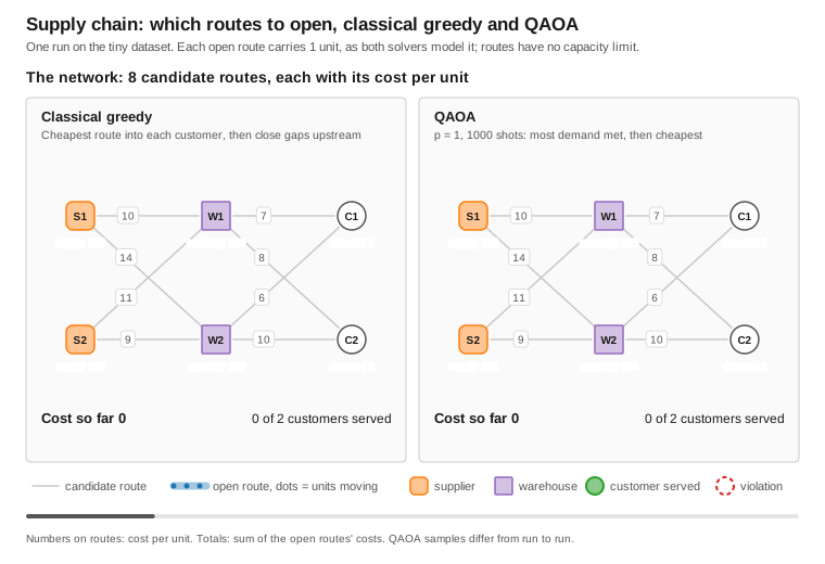
Network Flow
Use Case: Supply chain optimization, logistics, distribution planning
open System.Threading
open FSharp.Azure.Quantum

let nodes = [
    NetworkFlow.createSource "Factory" 100 100   // id, supply, capacity
    NetworkFlow.createIntermediate "Warehouse" 80
    NetworkFlow.createSink "Store1" 40           // id, demand
    NetworkFlow.createSink "Store2" 60
]

let routes = [
    NetworkFlow.createRoute "Factory" "Warehouse" 5.0   // from, to, cost
    NetworkFlow.createRoute "Warehouse" "Store1" 3.0
    NetworkFlow.createRoute "Warehouse" "Store2" 4.0
]

let problem = NetworkFlow.createProblem nodes routes

// Pass Some backend to run on quantum hardware/simulator; None uses the default.
task {
    match! NetworkFlow.solveAsync problem None CancellationToken.None with
    | Ok flow ->
        printfn "Total cost: $%.2f" flow.TotalCost
        printfn "Fill rate: %.1f%%" (flow.FillRate * 100.0)
    | Error err -> printfn "Error: %A" err
}
Task Scheduling
Use Case: Manufacturing workflows, project management, resource allocation with dependencies
open System.Threading
open FSharp.Azure.Quantum
open FSharp.Azure.Quantum.TaskScheduling
open FSharp.Azure.Quantum.Core.BackendAbstraction
open FSharp.Azure.Quantum.Backends.LocalBackend

// Define tasks with dependencies (durations and deadlines are TimeSpan values)
let taskA : ScheduledTask<unit> = scheduledTask {
    taskId "TaskA"
    duration (hours 2.0)
    priority 10.0
}

let taskB : ScheduledTask<unit> = scheduledTask {
    taskId "TaskB"
    duration (hours 1.5)
    after "TaskA"  // Dependency
    requires "Worker" 2.0
    deadline (minutes 240.0)
}

let taskC : ScheduledTask<unit> = scheduledTask {
    taskId "TaskC"
    duration (minutes 30.0)
    after "TaskA"
    requires "Machine" 1.0
}

// Define resources
let worker : Resource<unit> = resource {
    resourceId "Worker"
    capacity 3.0
}

let machine : Resource<unit> = resource {
    resourceId "Machine"
    capacity 2.0
}

// Build scheduling problem
let problem = scheduling {
    tasks [taskA; taskB; taskC]
    resources [worker; machine]
    objective MinimizeMakespan
    timeHorizon (hours 4.0)   // Keep close to the expected makespan; it sets the time-slot grid
}

// Solve with a quantum backend (qubits = tasks x time slots)
let backend = LocalBackend() :> IQuantumBackend

task {
    match! solveQuantumAsync backend problem CancellationToken.None with
    | Ok solution ->
        printfn "Makespan: %.2f hours" solution.Makespan.TotalHours
        solution.Assignments
        |> List.iter (fun assignment ->
            printfn "%s: starts %O, ends %O"
                assignment.TaskId assignment.StartTime assignment.EndTime)
    | Error err -> printfn "Error: %s" err.Message
}
Features:
- Dependency Management - Precedence constraints (task A before task B)
- Resource Constraints - Limited workers, machines, budget
- Quantum Optimization - QAOA for resource-constrained scheduling (
solveQuantumAsync) - Classical scheduler -
ClassicalSolver.solvefor dependency-only problems (ignores resource capacity) - Gantt Chart Export -
exportGanttChart solution "schedule.txt"
API Documentation: TaskScheduling-API.md
Examples:
- JobScheduling - Manufacturing workflow scheduling
Advanced Quantum Builders
High-level builders for specialized quantum algorithms using computation expression syntax.
Beyond the optimization builders, the library provides six advanced builders for specialized quantum computing tasks:
Quantum Tree Search Builder
Use Case: Graph traversal, decision trees, game tree exploration
open FSharp.Azure.Quantum

// Search a decision tree with Grover search (quantum search speedup)
let searchProblem = QuantumTreeSearch.quantumTreeSearch {
    initialState [0]                                        // Root state
    maxDepth 5                                              // Tree depth
    branchingFactor 3                                       // Children per node
    evaluateWith (fun state -> float (List.sum state))     // Score a state
    generateMovesWith (fun state -> [ for c in 1..3 -> state @ [c] ])  // Expand a node
}

match QuantumTreeSearch.solve searchProblem with
| Ok result ->
    printfn "Best move: %d" result.BestMove
    printfn "Score: %.4f" result.Score
    printfn "Paths explored: %d" result.PathsExplored
    printfn "Quantum advantage: %b" result.QuantumAdvantage
| Error err ->
    printfn "Error: %A" err
Features:
- Grover search over tree paths
- Amplitude amplification for target finding
- F# computation expression:
QuantumTreeSearch.quantumTreeSearch { } - Applications: Game AI, route planning, decision analysis
Quantum Constraint Solver Builder
Use Case: SAT solving, constraint satisfaction problems, logic puzzles
open FSharp.Azure.Quantum

// Solve a constraint-satisfaction problem (here: a 3-variable "all different")
let satProblem = QuantumConstraintSolver.constraintSolver {
    searchSpace 3                          // Number of variables (indices 0..2)
    domain [0; 1; 2]                       // Value each variable may take
    satisfies (fun assignment ->           // True when all constraints hold
        assignment.[0] <> assignment.[1] &&
        assignment.[1] <> assignment.[2] &&
        assignment.[0] <> assignment.[2])
}

match QuantumConstraintSolver.solve satProblem with
| Ok solution ->
    printfn "Satisfying assignment:"
    solution.Assignment
    |> Map.iter (fun var value -> printfn "  var%d = %A" var value)
    printfn "All constraints satisfied: %b" solution.AllConstraintsSatisfied
    printfn "Success probability: %.2f%%" (solution.SuccessProbability * 100.0)
| Error err ->
    printfn "Error: %A" err
Features:
- Grover-based constraint satisfaction
- Constraints given as ordinary F# predicates (
satisfies) - F# computation expression:
QuantumConstraintSolver.constraintSolver { } - Applications: Circuit verification, scheduling, logic puzzles
Quantum Pattern Matcher Builder
Use Case: String matching, DNA sequence alignment, anomaly detection
open FSharp.Azure.Quantum

// Find the items matching a predicate, with quantum search speedup (Grover)
let matchProblem = QuantumPatternMatcher.patternMatcher {
    searchSpace [1; 2; 3; 4; 5; 6; 7; 8]   // Candidate items
    matchPattern (fun x -> x % 3 = 0)      // Pattern: multiples of 3
    findTop 2                              // Return up to 2 matches
}

match QuantumPatternMatcher.solve matchProblem with
| Ok result ->
    printfn "Matches found: %A" result.Matches
    printfn "Search space size: %d" result.SearchSpaceSize
    printfn "Success probability: %.2f%%" (result.SuccessProbability * 100.0)
| Error err ->
    printfn "Error: %A" err
Features:
- Grover search for items matching a predicate
- Return the top matches (
findTop) - F# computation expression:
QuantumPatternMatcher.patternMatcher { } - Applications: Bioinformatics, data mining, signal processing
Quantum Arithmetic Builder
Use Case: Cryptographic operations, RSA encryption, modular arithmetic
open FSharp.Azure.Quantum

// Quantum integer addition: 15 + 27
let addProblem = QuantumArithmeticOps.quantumArithmetic {
    operands 15 27
    operation QuantumArithmeticOps.Add
    qubits 10
}

// The CE returns a validated Result<ArithmeticOperation, _>; bind, then execute.
match addProblem with
| Ok op ->
    match QuantumArithmeticOps.execute op with
    | Ok result ->
        printfn "Result: %d" result.Value
        printfn "Gates used: %d" result.GateCount
        printfn "Circuit depth: %d" result.CircuitDepth
        printfn "Modular: %b" result.IsModular
    | Error err -> printfn "Error: %A" err
| Error err -> printfn "Error: %A" err

// Modular exponentiation for RSA: 5^3 mod 33
let rsaProblem = QuantumArithmeticOps.quantumArithmetic {
    operands 5 3                                // base = 5, exponent = 3
    operation QuantumArithmeticOps.ModularExponentiate
    modulus 33                                  // RSA modulus
    qubits 6                                    // register; the circuit takes 2·6 + 5 = 17 qubits
}
Features:
- Quantum arithmetic operations (Add, Subtract, Multiply, ModularExponentiate)
- QFT-based carry propagation
- F# computation expression:
QuantumArithmeticOps.quantumArithmetic { } - Applications: Cryptography, financial calculations, scientific computing
Quantum Period Finder Builder
Use Case: Shor's algorithm, cryptanalysis, order finding
open FSharp.Azure.Quantum

// Find the period of a modular function (core of Shor's algorithm)
let shorsProblem = QuantumPeriodFinder.periodFinder {
    number 15                   // Composite to factor
    chosenBase 7                // Coprime base
    precision 12                // QPE precision bits requested; N = 15 runs with 8 on the default 20-qubit budget
    maxAttempts 10              // Probabilistic retries
}

// The CE returns a validated Result<PeriodFinderProblem, _>; bind, then solve.
match shorsProblem with
| Ok problem ->
    match QuantumPeriodFinder.solve problem with
    | Ok result ->
        printfn "Period found: %d" result.Period
        match result.Factors with
        | Some (p, q) ->
            printfn "Factors: %d x %d = %d" p q (p * q)
            printfn "RSA modulus factored!"
        | None ->
            printfn "Retry with a different base (probabilistic)"
    | Error err -> printfn "Error: %A" err
| Error err -> printfn "Error: %A" err
Features:
- Quantum Period Finding (QPF) for Shor's algorithm
- Quantum Phase Estimation (QPE) integration
FactorSourcesays how the factors were found:QuantumPeriodFinding(from the measured period) orClassicalPreprocessing(N even, or the base shares a factor with N, so no circuit ran)- F# computation expression:
QuantumPeriodFinder.periodFinder { } - Applications: Cryptanalysis, number theory, discrete logarithm
Quantum Phase Estimator Builder
Use Case: Eigenvalue estimation, quantum chemistry, VQE enhancement
open System
open FSharp.Azure.Quantum
// UnitaryOperator (RotationZ, PhaseGate, ...)
open FSharp.Azure.Quantum.Algorithms.QPE

// Estimate the eigenphase of a unitary operator
let qpeProblem = QuantumPhaseEstimator.phaseEstimator {
    unitary (RotationZ (Math.PI / 4.0))   // Operator U
    precision 16                          // 16-bit phase precision
    targetQubits 1
}

// The CE returns a validated Result<PhaseEstimatorProblem, _>; bind, then estimate.
match qpeProblem with
| Ok problem ->
    match QuantumPhaseEstimator.estimate problem with
    | Ok result ->
        printfn "Estimated phase: %.6f" result.Phase
        printfn "Eigenvalue: %A" result.Eigenvalue
        printfn "Measurement outcome: %d" result.MeasurementOutcome
        printfn "Eigenphase angle: %.4f rad" (result.Phase * 2.0 * Math.PI)
    | Error err -> printfn "Error: %A" err
| Error err -> printfn "Error: %A" err
Features:
- Quantum Phase Estimation (QPE) with arbitrary precision
- Inverse QFT for phase readout
- F# computation expression:
QuantumPhaseEstimator.phaseEstimator { } - Applications: Quantum chemistry (VQE), linear systems, machine learning
Advanced Builder Features
Common Capabilities:
- Computation Expression Syntax - Idiomatic F# DSL for all builders
- Backend Switching - LocalBackend (simulation) or Cloud (IonQ, Rigetti, Quantinuum, Atom Computing, IQM): on a cloud backend each run is submitted as one whole-circuit job, and the results come from measured shots
- Type Safety - F# type system prevents invalid quantum circuits
- C# Interop - Fluent API extensions for all builders
- Circuit Export - Export to OpenQASM 2.0 for cross-platform execution
- Error Handling - Comprehensive validation and error messages
Current Status:
- Educational/Research Focus - Suitable for algorithm learning and prototyping
- NISQ Limitations - Toy problems only (about 20 qubits) on current hardware and the local simulator
- Production-Quality Code - Well-tested, documented, and production-quality implementation
- Hardware Bottleneck - Waiting for fault-tolerant quantum computers for real-world scale
Use Cases by Builder:
| Builder | Primary Application | Underlying Algorithm | Theoretical Speedup |
|---|---|---|---|
| Tree Search | Game AI, Route Planning | Grover search over paths | O(√N) |
| Constraint Solver | SAT, Logic Puzzles | Grover search over assignments | O(√2^n) |
| Pattern Matcher | DNA Alignment, Data Mining | Grover search over candidates | O(√N) |
| Arithmetic | Cryptography, RSA | QFT-based arithmetic | None on its own (QFT-based adders are the building block of Shor's modular exponentiation) |
| Period Finder | Shor's Algorithm, Cryptanalysis | Quantum phase estimation | Exponential |
| Phase Estimator | Quantum Chemistry, VQE | Quantum phase estimation | Polynomial |
Recommendation:
- Use for learning quantum algorithms and understanding quantum advantage
- Use for prototyping future quantum applications
- For production optimization, use the 7 problem builders instead
C# API for Advanced Builders
All advanced builders have C#-friendly fluent APIs:
using System;
using FSharp.Azure.Quantum;
using static FSharp.Azure.Quantum.CSharpBuilders;

// Tree Search: initial state, scoring function, and move generator
var treeSearch = QuantumTreeSearch(
    initialState: 0,
    evaluator: x => (double)x,
    moveGenerator: x => new[] { x + 1, x + 2 });
var searchResult = SolveTreeSearch(treeSearch);

// Constraint Solver: number of variables, domain, and a constraint predicate
var satProblem = QuantumConstraintSolver(
    searchSpaceSize: 3,
    domain: new[] { 0, 1 },
    singleConstraint: assignment => assignment[0] != assignment[1]);
var satResult = SolveConstraints(satProblem);

// Pattern Matcher: candidate configurations and a match predicate
var pattern = QuantumPatternMatcher(
    configurations: new[] { 1, 2, 3, 4, 5, 6, 7, 8 },
    pattern: x => x % 3 == 0);
var matchResult = SolvePatternMatch(pattern);

// Arithmetic: build an operation, then execute it
var add = Add(15, 27);
var addResult = ExecuteArithmetic(add);

var rsa = ModularExponentiate(baseValue: 5, exponent: 3, modulus: 33);
var rsaResult = ExecuteArithmetic(rsa);

// Period Finder (Shor's): the factory returns a Result; unwrap before executing. N = 15 runs with 8 counting qubits on the default 20-qubit budget
var shors = FactorInteger(15, precision: 12);
if (shors.IsOk)
{
    var factorResult = ExecutePeriodFinder(shors.ResultValue);
}

// Phase Estimator: EstimateRotationZ also returns a Result
var qpe = EstimateRotationZ(Math.PI / 4.0, precision: 16);
if (qpe.IsOk)
{
    var phaseResult = ExecutePhaseEstimator(qpe.ResultValue);
}
Current Status: Educational/research focus - Demonstrates quantum algorithms, but current hardware is insufficient for real-world sizes (fault-tolerant hardware needed)
Library Scope & Focus
Primary Focus: QAOA-Based Combinatorial Optimization
This library is designed for QAOA-based combinatorial optimization:
- ✅ 7 optimization problem builders (Graph Coloring, MaxCut, TSP, Knapsack, Portfolio, Network Flow, Task Scheduling)
- ✅ QAOA implementation with automatic parameter tuning
- ✅ Error mitigation for noisy hardware (ZNE, PEC, REM)
- ✅ Production-ready solvers with cloud backend integration (local simulator by default)
Secondary Focus: Quantum Algorithm Education & Research
The Algorithms/ directory contains foundational quantum algorithms for learning:
- ✅ Grover's Search (quantum search, O(√N) speedup)
- ✅ Amplitude Amplification (generalization of Grover)
- ✅ Quantum Fourier Transform (O(n²) gates vs O(n·2^n) for the classical FFT)
Why F# for Quantum?
- Type-safe quantum circuit construction
- Functional programming matches quantum mathematics
- Interop with .NET ecosystem (C#, Azure, ML.NET)
- Higher level abstraction than Python (Qiskit) and Q#: problem builders and computation expressions instead of hand-built circuits
Quantum Machine Learning (QML)
Apply quantum computing to machine learning problems with variational quantum circuits and quantum kernels.
Variational Quantum Classifier (VQC)
Train quantum neural networks for classification tasks:
open System.Threading
open FSharp.Azure.Quantum.Core.BackendAbstraction
open FSharp.Azure.Quantum.Backends.LocalBackend
open FSharp.Azure.Quantum.MachineLearning

// Setup backend and architecture
let backend = LocalBackend() :> IQuantumBackend
let featureMap = AngleEncoding
let variationalForm = RealAmplitudes 2  // 2 layers

// Prepare training data (features and labels as separate arrays)
let trainFeatures = [|
    [| 0.1; 0.2 |]
    [| 0.9; 0.8 |]
    [| 0.3; 0.1 |]
    [| 0.8; 0.9 |]
|]
let trainLabels = [| 0; 1; 0; 1 |]

// Configure training (start from the defaults and override what you need)
let config : VQC.TrainingConfig = {
    VQC.defaultConfig with
        LearningRate = 0.1
        MaxEpochs = 100
        ConvergenceThreshold = 0.001
        Shots = 1000
        Verbose = false
        Optimizer = VQC.SGD
}

// Initialize parameters (one qubit per feature)
let numQubits = trainFeatures.[0].Length
let initialParams = VariationalForms.randomParameters variationalForm numQubits (Some 42)

// Train the classifier
task {
    match! VQC.trainAsync backend featureMap variationalForm initialParams trainFeatures trainLabels config CancellationToken.None with
    | Ok result ->
        // Make predictions
        let testPoint = [| 0.5; 0.5 |]
        match! VQC.predictAsync backend featureMap variationalForm result.Parameters testPoint 1000 CancellationToken.None with
        | Ok prediction ->
            printfn "Prediction: %d (probability: %.2f%%)"
                prediction.Label (prediction.Probability * 100.0)
        | Error err -> printfn "Error: %s" err.Message
    | Error err -> printfn "Training failed: %s" err.Message
}
Quantum Kernel SVM
Use quantum feature spaces for support vector machines:
open System.Threading
open FSharp.Azure.Quantum.Core.BackendAbstraction
open FSharp.Azure.Quantum.Backends.LocalBackend
open FSharp.Azure.Quantum.MachineLearning

// Setup backend and quantum feature map
let backend = LocalBackend() :> IQuantumBackend
let featureMap = ZZFeatureMap 2  // Depth-2 entangling feature map

// Training data
let trainData = [| [| 0.1; 0.2 |]; [| 0.9; 0.8 |]; [| 0.3; 0.1 |]; [| 0.8; 0.9 |] |]
let trainLabels = [| 0; 1; 0; 1 |]

// SVM configuration
let config : QuantumKernelSVM.SVMConfig = {
    QuantumKernelSVM.defaultConfig with
        C = 1.0
        Tolerance = 1e-3
        MaxIterations = 100
        Verbose = false
}

// Train SVM with quantum kernel
task {
    match! QuantumKernelSVM.trainAsync backend featureMap trainData trainLabels config 1000 CancellationToken.None with
    | Ok model ->
        // Evaluate on test data
        let testData = [| [| 0.5; 0.5 |]; [| 0.2; 0.8 |] |]
        let testLabels = [| 0; 1 |]

        match! QuantumKernelSVM.evaluateAsync backend model testData testLabels 1000 CancellationToken.None with
        | Ok accuracy -> printfn "Test accuracy: %.2f%%" (accuracy * 100.0)
        | Error err -> printfn "Evaluation error: %s" err.Message
    | Error err -> printfn "Training error: %s" err.Message
}
QML Features:
- VQC - Variational quantum circuits for supervised learning
- Quantum Kernels - Leverage quantum feature spaces in SVMs
- Feature Maps - ZZFeatureMap, PauliFeatureMap for encoding classical data
- Variational Forms - RealAmplitudes, EfficientSU2 ansatz circuits
- Adam Optimizer - Gradient-based training with momentum
- Model Serialization - Save/load trained models
- Data Preprocessing - Normalization, encoding, splits
The same code runs on a cloud backend: every forward pass and every kernel entry is one circuit submitted with ExecuteToState, so training is many billed jobs (a kernel matrix of n samples is n(n+1)/2 circuits). Kernel matrices keep at most QuantumKernels.MaxConcurrentSampledJobs (8) circuits in flight on a cloud backend; cap the total with a JobBudget.
Examples:
examples/QML/VQCExample.fsx- Complete VQC training pipelineexamples/QML/FeatureMapExample.fsx- Feature encoding demonstrationsexamples/QML/VariationalFormExample.fsx- Ansatz circuit exploration
Business Problem Builders
High-level APIs for common business applications powered by quantum algorithms (Grover's search) and quantum machine learning.
Social Network Analyzer - Community Detection & Fraud Rings
Use Grover's algorithm to find tight-knit communities (cliques) in social networks for marketing, fraud detection, and team analysis.
open FSharp.Azure.Quantum.Business
open FSharp.Azure.Quantum.Core.BackendAbstraction
open FSharp.Azure.Quantum.Backends.LocalBackend

// Define social network
let network = SocialNetworkAnalyzer.socialNetwork {
    // Add people
    people ["Alice"; "Bob"; "Carol"; "Dave"; "Eve"; "Frank"]

    // Define connections (friendships, transactions, communications)
    connections [
        ("Alice", "Bob")
        ("Bob", "Carol")
        ("Carol", "Alice")     // Triangle: potential community

        ("Dave", "Eve")
        ("Eve", "Frank")
        ("Frank", "Dave")      // Another triangle

        ("Carol", "Dave")      // Bridge between communities
    ]

    // Find communities of at least 3 people
    findCommunities 3

    // Backend is optional; the local simulator is used when omitted
    backend (LocalBackend() :> IQuantumBackend)
    shots 1000
}

task {
    match! network with
    | Ok result ->
        printfn "Communities found: %d" result.Communities.Length

        for comm in result.Communities do
            printfn "Community: %A" comm.Members
            printfn "  Strength: %.0f%% connected" (comm.Strength * 100.0)
            printfn "  Internal connections: %d" comm.InternalConnections
    | Error err -> printfn "Error: %A" err
}
Business Use Cases:
- Marketing: Identify influencer groups for targeted campaigns
- Fraud Detection: Detect fraud rings through circular transaction patterns
- HR Analytics: Analyze team collaboration and communication networks
- Healthcare: Track disease outbreak clusters and contact tracing
- Security: Find coordinated bot networks or insider threat groups
Quantum Advantage:
- Classical clique finding: O(2^n) exponential time complexity
- Grover's algorithm: O(√(2^n)) quadratic speedup (theoretical; about √(2^n) oracle queries)
How it works:
- Clique search is encoded as a Grover search over subsets of people (
useQaoaswitches to a QAOA formulation where supported) - The Grover search needs one qubit per person, up to what the backend runs; the QAOA formulations split wider networks where the settings allow
Features:
- F# computation expression:
socialNetwork { } - Quantum backend support (LocalBackend by default, or any gate-based cloud backend: every Grover or QAOA circuit is submitted as one whole-circuit job)
- Configurable shots for measurement accuracy
- Community strength metrics (connectivity percentage)
Example: examples/GraphAnalytics/SocialNetworkAnalyzer_Example.fsx
Constraint Scheduler - Workforce & Resource Allocation
Use quantum optimization (Max-SAT and Weighted Graph Coloring) to solve scheduling problems with hard and soft constraints.
open FSharp.Azure.Quantum.Business
open FSharp.Azure.Quantum.Core.BackendAbstraction
open FSharp.Azure.Quantum.Backends.LocalBackend

// Workforce scheduling with constraints
let schedule = ConstraintScheduler.constraintScheduler {
    // Define shifts to cover
    task "Morning"
    task "Afternoon"
    task "Evening"
    task "Night"

    // Available workers with hourly rates
    resource "Alice" 25.0   // Senior: $25/hour
    resource "Bob" 15.0     // Junior: $15/hour
    resource "Carol" 20.0   // Mid-level: $20/hour
    resource "Dave" 15.0    // Junior: $15/hour

    // Hard constraints (MUST be satisfied)
    conflict "Morning" "Afternoon"     // Can't work consecutive shifts
    conflict "Afternoon" "Evening"
    conflict "Evening" "Night"

    // Soft constraints (preferences with weights)
    prefer "Morning" "Alice" 10.0      // Alice prefers morning
    prefer "Afternoon" "Carol" 8.0     // Carol prefers afternoon
    prefer "Night" "Dave" 9.0          // Dave prefers night

    // Optimization goal
    optimizeFor ConstraintScheduler.MinimizeCost
    maxBudget 100.0

    // Backend is optional; the local simulator is used when omitted
    backend (LocalBackend() :> IQuantumBackend)
    shots 1500
}

task {
    match! schedule with
    | Ok result ->
        match result.BestSchedule with
        | Some sched ->
            printfn "Optimal Shift Assignments:"
            for assignment in sched.Assignments do
                printfn "  %s → %s ($%.2f/hour)"
                    assignment.Task
                    assignment.Resource
                    assignment.Cost

            printfn "\nTotal Cost: $%.2f" sched.TotalCost
            printfn "Constraints Satisfied: %d / %d hard, %d / %d soft"
                sched.HardConstraintsSatisfied
                sched.TotalHardConstraints
                sched.SoftConstraintsSatisfied
                sched.TotalSoftConstraints
            printfn "Feasible: %b" sched.IsFeasible
        | None ->
            printfn "No feasible schedule found"
    | Error err -> printfn "Error: %A" err
}
Business Use Cases:
- Workforce Management: Employee shift scheduling with availability constraints
- Cloud Computing: VM allocation to minimize costs while meeting SLAs
- Manufacturing: Production task assignment with equipment constraints
- Logistics: Delivery route optimization with time windows
- Project Management: Task assignment with dependencies and deadlines
Quantum Advantage:
- Classical constraint solving: NP-hard (exponential time)
- Quantum optimization: Quadratic speedup with Grover search (theoretical)
Optimization Goals:
MinimizeCost: Uses Weighted Graph Coloring oracle (when resources have capacities: QAOA on a task-resource assignment QUBO with each resource's own capacity, the hard constraints and the costs)MaximizeSatisfaction: Uses Max-SAT oracle for constraint satisfactionBalanced: Combines both cost and satisfaction criteria
Constraint Types:
- Hard Constraints (must satisfy):
conflict,require.precedenceis rejected with an error: this scheduler assigns tasks to resources and has no time dimension (use Task Scheduling for ordering). - Soft Constraints (preferences):
preferwith configurable weights - Budget Constraints:
maxBudgetfor cost optimization
Features:
- F# computation expression:
constraintScheduler { } - Dual oracle support (Max-SAT and Weighted Graph Coloring)
- Quantum backend support (LocalBackend by default, or any gate-based cloud backend: every Grover or QAOA circuit is submitted as one whole-circuit job)
- Configurable shots for accuracy vs. speed tradeoff
- Up to 50 tasks accepted; when the quantum search finds no schedule,
BestScheduleisNone(no classical search runs in its place) - Detailed constraint satisfaction metrics
Example: examples/JobScheduling/ConstraintScheduler_Example.fsx
AutoML - Automated Machine Learning
open System.Threading
open FSharp.Azure.Quantum.Business

// Training data: each sample is a float array of features, with a numeric label
let features = [| [| 0.1; 0.2 |]; [| 0.9; 0.8 |]; [| 0.2; 0.1 |]; [| 0.8; 0.9 |] |]
let labels   = [| 0.0; 1.0; 0.0; 1.0 |]

// The CE runs the automated model search and returns Task<QuantumResult<AutoMLResult>>
task {
    let! automlResult =
        AutoML.autoML {
            trainWith features labels
            tryBinaryClassification true
            maxTrials 20
            validationSplit 0.2
        }

    match automlResult with
    | Ok result ->
        printfn "Best model: %s (validation score %.2f%%)" result.BestModelType (result.Score * 100.0)
        printfn "Best architecture: %A" result.BestArchitecture

        // Use the best model for a prediction
        match! AutoML.predictAsync [| 0.85; 0.85 |] result CancellationToken.None with
        | Ok prediction -> printfn "Prediction: %A" prediction
        | Error err -> printfn "Error: %A" err
    | Error err -> printfn "Error: %A" err
}
Anomaly Detection - Security & Fraud Detection
open System.Threading
open FSharp.Azure.Quantum.Business

// Train on NORMAL examples only (one-class anomaly detection).
// Each sample is a float array of features (packet size, duration, failed logins).
let normalTraffic =
    [| [| 0.10; 0.20; 0.0 |]
       [| 0.15; 0.25; 0.0 |]
       [| 0.12; 0.18; 0.1 |] |]

// The CE trains the detector and returns Task<QuantumResult<Detector>>
task {
    let! detectorResult =
        AnomalyDetector.anomalyDetection {
            trainOnNormalData normalTraffic
            sensitivity AnomalyDetector.High
            contaminationRate 0.05
        }

    match detectorResult with
    | Ok detector ->
        // Score a new sample against the trained detector
        let sample = [| 0.9; 0.95; 0.8 |]
        match! AnomalyDetector.checkAsync sample detector CancellationToken.None with
        | Ok result ->
            printfn "Anomaly: %b (score %.3f)" result.IsAnomaly result.AnomalyScore
        | Error err -> printfn "Error: %A" err
    | Error err -> printfn "Error: %A" err
}
Binary Classification - Fraud Detection
open System.Threading
open FSharp.Azure.Quantum.Business

// Labeled transactions: features as float arrays, labels 0 = legitimate, 1 = fraud
let trainX = [| [| 0.1; 0.2 |]; [| 0.9; 0.8 |]; [| 0.2; 0.1 |]; [| 0.85; 0.9 |] |]
let trainY = [| 0; 1; 0; 1 |]

// The CE trains the classifier and returns Task<QuantumResult<Classifier>>
task {
    let! classifierResult =
        BinaryClassifier.binaryClassification {
            trainWith trainX trainY
            architecture BinaryClassifier.Hybrid   // Quantum feature map + classical SVM
            maxEpochs 50
        }

    match classifierResult with
    | Ok model ->
        // Evaluate on held-out data (features, labels, classifier)
        let testX = [| [| 0.15; 0.2 |]; [| 0.8; 0.85 |] |]
        let testY = [| 0; 1 |]
        match! BinaryClassifier.evaluateAsync testX testY model CancellationToken.None with
        | Ok metrics ->
            printfn "Precision: %.2f%%" (metrics.Precision * 100.0)
            printfn "Recall: %.2f%%" (metrics.Recall * 100.0)
            printfn "F1 Score: %.2f" metrics.F1Score
        | Error err -> printfn "Error: %A" err

        // Classify a new sample
        match! BinaryClassifier.predictAsync [| 0.82; 0.88 |] model CancellationToken.None with
        | Ok prediction ->
            printfn "Label: %d (%.2f%% confidence)" prediction.Label (prediction.Confidence * 100.0)
        | Error err -> printfn "Error: %A" err
    | Error err -> printfn "Training failed: %A" err
}
Predictive Modeling - Customer Churn Prediction
open System.Threading
open FSharp.Azure.Quantum.Business

// Historical customers: features (e.g. tenure, monthly charges), target = churn score
let history = [| [| 12.0; 50.0 |]; [| 1.0; 90.0 |]; [| 24.0; 40.0 |]; [| 2.0; 95.0 |] |]
let targets = [| 0.0; 1.0; 0.0; 1.0 |]

// The CE trains the model and returns Task<QuantumResult<Model>>
task {
    let! modelResult =
        PredictiveModel.predictiveModel {
            trainWith history targets
            problemType PredictiveModel.Regression
            architecture PredictiveModel.Hybrid
            maxEpochs 50
        }

    match modelResult with
    | Ok model ->
        // Score an active customer (backend / shots optional -> None None uses defaults)
        match! PredictiveModel.predictAsync [| 3.0; 92.0 |] model None None CancellationToken.None with
        | Ok prediction -> printfn "Predicted churn score: %.3f" prediction.Value
        | Error err -> printfn "Error: %A" err
    | Error err -> printfn "Error: %A" err
}
Similarity Search - Product Recommendations
Build a SearchIndex from a catalog with similaritySearch { ... }, then rank
neighbours with SimilaritySearch.findSimilarAsync queryItem queryFeatures topN index cancellationToken
(returns Task<QuantumResult<SearchResults<'T>>>).
▶ Full runnable example: examples/SimilaritySearch/ProductRecommendations.fsx
Business Builder Features:
- Social Network Analyzer - Community detection, fraud rings, influencer identification (Grover's algorithm)
- Constraint Scheduler - Workforce scheduling, resource allocation with constraints (Max-SAT & Graph Coloring)
- AutoML - Automated model and architecture search with hyperparameter trials
- Anomaly Detection - Outlier detection for security, fraud, quality control
- Binary Classification - Two-class problems (fraud, spam, churn)
- Predictive Modeling - Regression and multi-class prediction (demand, churn)
- Similarity Search - Recommendations, semantic search, clustering
- Quantum-Enhanced - Uses Grover's search, quantum kernels, and feature maps
- Ready for Production - Model serialization, evaluation metrics, validation
Examples:
examples/GraphAnalytics/SocialNetworkAnalyzer_Example.fsx- Community detection and fraud ring identificationexamples/JobScheduling/ConstraintScheduler_Example.fsx- Workforce and resource schedulingexamples/AutoML/QuickPrototyping.fsx- Complete AutoML pipelineexamples/AnomalyDetection/SecurityThreatDetection.fsx- Network security monitoringexamples/BinaryClassification/FraudDetection.fsx- Transaction fraud detectionexamples/PredictiveModeling/CustomerChurnPrediction.fsx- Churn predictionexamples/SimilaritySearch/ProductRecommendations.fsx- E-commerce recommendations
HybridSolver - Automatic Classical/Quantum Routing
Smart solver that automatically chooses between classical and quantum execution based on problem analysis.
The HybridSolver provides a unified API that:
- Analyzes problem size (
ProblemAnalysis) - Estimates quantum advantage potential (
QuantumAdvisor: estimated speedup and classical/quantum solving times) - Routes to a classical solver (fast, free) or to a quantum solver on the backend you pass
- Records the reasoning for its choice in the result
- Accepts an optional budget (USD) that sends a problem back to the classical solver when the estimated quantum cost exceeds it
Decision Framework (QuantumAdvisor.defaultThresholds):
- Small problems (below 50 variables) → classical solver (milliseconds, $0)
- Large problems (50 variables or more) → quantum solver (seconds to minutes, provider pricing), only if you passed a backend (the
...WithBackendAsyncfunctions) and the estimated cost is within the budget; otherwise the classical solver runs andReasoningsays why - Automatic cost guards and recommendations: the cost of a QAOA run is estimated with
CostEstimationfrom the backend name (IonQ: $12.42 base per job, $97.50 with error mitigation, plus per-gate-per-shot charges; Rigetti: $0.02 per 10 ms of QPU time; Quantinuum: subscription-priced; simulators: free). For the one-layer, 1000-shot QAOA circuit HybridSolver prices, a 10-variable problem estimates at about $60 on IonQ and a 50-variable problem at about $1,230, so set a budget before routing large problems to paid hardware. forceMethod = Some Classical/Some Quantumbypasses the advisor (forced quantum uses the given backend, or a new LocalBackend)
Supported Problems
The HybridSolver supports five optimization problems: TSP, Portfolio, MaxCut, Knapsack and Graph Coloring. MaxCut, Knapsack and Graph Coloring take the solver-level problem records from FSharp.Azure.Quantum.Quantum.
open System.Threading
open FSharp.Azure.Quantum
open FSharp.Azure.Quantum.Quantum
open FSharp.Azure.Quantum.Classical
open FSharp.Azure.Quantum.Core.BackendAbstraction
open FSharp.Azure.Quantum.Backends.LocalBackend

// TSP with automatic routing
let distances = array2D [[0.0; 10.0; 15.0];
                          [10.0; 0.0; 20.0];
                          [15.0; 20.0; 0.0]]

task {
    match! HybridSolver.solveTspAsync distances None None None CancellationToken.None with
    | Ok solution ->
        printfn "Method used: %A" solution.Method           // Classical or Quantum
        printfn "Reasoning: %s" solution.Reasoning          // Why this method?
        printfn "Time: %.2f ms" solution.ElapsedMs
        printfn "Tour: %A" solution.Result.Tour
        printfn "Length: %.2f" solution.Result.TourLength
    | Error err -> printfn "Error: %s" err.Message
}

// MaxCut: convert the builder problem to the solver-level record
let maxCutProblem = MaxCut.createProblem ["A"; "B"; "C"; "D"] [("A", "B", 1.0); ("B", "C", 2.0); ("C", "D", 1.0)]
let hybridMaxCut : QuantumMaxCutSolver.MaxCutProblem =
    { Vertices = maxCutProblem.Vertices; Edges = maxCutProblem.Edges }

// Pass a backend so that large problems can run on it; budget = Some 50.0 USD
let backend = LocalBackend() :> IQuantumBackend
task {
    match! HybridSolver.solveMaxCutWithBackendAsync hybridMaxCut (Some 50.0) None None (Some backend) CancellationToken.None with
    | Ok solution ->
        printfn "Method: %A" solution.Method
        printfn "Cut Value: %.2f" solution.Result.CutValue
        match solution.Recommendation with
        | Some recommendation -> printfn "Advisor: %s" recommendation.Reasoning
        | None -> ()
    | Error err -> printfn "Error: %s" err.Message
}

// Knapsack
let knapsack = Knapsack.createProblem [("laptop", 3.0, 1000.0); ("phone", 0.5, 500.0); ("tablet", 1.5, 700.0)] 4.0
let knapsackProblem : QuantumKnapsackSolver.KnapsackProblem =
    { Items = knapsack.Items; Capacity = knapsack.Capacity }

task {
    match! HybridSolver.solveKnapsackAsync knapsackProblem None None None CancellationToken.None with
    | Ok solution ->
        printfn "Total Value: %.2f" solution.Result.TotalValue
        printfn "Items: %A" (solution.Result.SelectedItems |> List.map (fun i -> i.Id))
    | Error err -> printfn "Error: %s" err.Message
}

// Graph Coloring
let graphProblem : QuantumGraphColoringSolver.GraphColoringProblem = {
    Vertices = ["R1"; "R2"; "R3"]
    Edges = [ GraphOptimization.edge "R1" "R2" 1.0; GraphOptimization.edge "R2" "R3" 1.0 ]
    NumColors = 3
    FixedColors = Map.empty
}

task {
    match! HybridSolver.solveGraphColoringAsync graphProblem 3 None None None CancellationToken.None with
    | Ok solution ->
        printfn "Colors Used: %d/3" solution.Result.ColorsUsed
        printfn "Valid: %b" solution.Result.IsValid
    | Error err -> printfn "Error: %s" err.Message
}

// Portfolio Optimization
let assets : PortfolioSolver.Asset list = [
    { Symbol = "AAPL"; ExpectedReturn = 0.12; Risk = 0.15; Price = 150.0 }
    { Symbol = "MSFT"; ExpectedReturn = 0.11; Risk = 0.14; Price = 350.0 }
]
let constraints : PortfolioSolver.Constraints = { Budget = 10000.0; MinHolding = 0.0; MaxHolding = 6000.0 }

task {
    match! HybridSolver.solvePortfolioAsync assets constraints None None None CancellationToken.None with
    | Ok solution ->
        printfn "Portfolio Value: $%.2f" solution.Result.TotalValue
        printfn "Expected Return: %.2f%%" (solution.Result.ExpectedReturn * 100.0)
    | Error err -> printfn "Error: %s" err.Message
}

// With a covariance matrix (validated) both paths report risk as sqrt(wᵀΣw)
let covariance = array2D [ [ 0.0225; 0.0126 ]; [ 0.0126; 0.0196 ] ]

task {
    match! HybridSolver.solvePortfolioWithCovarianceAsync assets covariance constraints None None None None CancellationToken.None with
    | Ok solution -> printfn "Risk: %.2f%%" (solution.Result.Risk * 100.0)
    | Error err -> printfn "Error: %s" err.Message
}
Features
- Unified API: Single function call for any problem size
- Smart Routing: Automatic classical/quantum decision (
QuantumAdvisorrecommendation, applied when a backend is supplied) - Cost Guards: the
budgetargument (USD) prevents runaway quantum costs by keeping expensive runs classical - Transparent Reasoning:
Solution.Reasoningexplains why each method was chosen - Quantum Advisor:
Solution.Recommendationcarries the advisor's recommendation, confidence and estimated speedup - Forced method:
Some HybridSolver.Classical/Some HybridSolver.Quantum
When to Use HybridSolver vs Direct Builders
Use HybridSolver when:
- Problem size varies (sometimes small, sometimes large)
- You want automatic cost optimization (small problems solved classically for free, a budget guard on quantum cost)
- You're prototyping and unsure which approach is better
Use Direct Builders when:
- You always want quantum (for research/learning)
- The problem fits the backend's qubit budget (LocalBackend: memory-derived, about 20 qubits for QAOA by default)
- You need fine-grained control over backend configuration
- You're integrating with specific QAOA parameter tuning
Location: src/FSharp.Azure.Quantum/Solvers/Hybrid/HybridSolver.fs
Status: Recommended for production deployments
Architecture
Intent-First Algorithms (Backend-Aware Planning)
Some algorithms (notably Grover-family building blocks such as Amplitude Amplification) are implemented as intent → plan → execute rather than as a single canonical gate circuit.
- On gate-native backends, this may lower to standard gate operations.
- On non-gate-native backends (e.g., topological models), the same intent can be executed with native semantic operations.
- If a backend can’t support an algorithm’s intent and there is no valid lowering, the library should fail explicitly rather than silently producing an incorrect result.
This is primarily a portability/correctness feature; most users won’t need to change code. Details: docs/adr-intent-first-algorithms.md.
3-Layer Quantum-Only Architecture
graph TB
    subgraph "Layer 1: High-Level Builders"
        GC["GraphColoring Builder<br/>graphColoring { }"]
        MC["MaxCut Builder<br/>MaxCut.createProblem"]
        KS["Knapsack Builder<br/>Knapsack.createProblem"]
        TS["TSP Builder<br/>TSP.createProblem"]
        PO["Portfolio Builder<br/>Portfolio.createProblem"]
        NF["NetworkFlow Builder<br/>NetworkFlow module"]
        SCHED["TaskScheduling Builder<br/>scheduledTask { }"]
    end

    subgraph "Layer 2: Quantum Solvers"
        QGC["QuantumGraphColoringSolver<br/>(QAOA)"]
        QMC["QuantumMaxCutSolver<br/>(QAOA)"]
        QKS["QuantumKnapsackSolver<br/>(QAOA)"]
        QTS["QuantumTspSolver<br/>(QAOA)"]
        QPO["QuantumPortfolioSolver<br/>(QAOA)"]
        QNF["QuantumNetworkFlowSolver<br/>(QAOA)"]
        QSCHED["TaskScheduling.QuantumSolver<br/>(QAOA)"]
    end

    subgraph "Layer 3: Quantum Backends"
        LOCAL["LocalBackend<br/>(memory-derived width)"]
        IONQ["IonQ cloud backend<br/>(Azure Quantum)"]
        RIGETTI["Rigetti cloud backend<br/>(Azure Quantum)"]
        ATOM["Atom Computing cloud backend<br/>(Azure Quantum, 100 qubits)"]
        QUANTINUUM["Quantinuum cloud backend<br/>(Azure Quantum, 99.9%+ fidelity)"]
    end

    GC --> QGC
    MC --> QMC
    KS --> QKS
    TS --> QTS
    PO --> QPO
    NF --> QNF
    SCHED --> QSCHED

    QGC --> LOCAL
    QMC --> LOCAL
    QKS --> LOCAL
    QTS --> LOCAL
    QPO --> LOCAL
    QNF --> LOCAL
    QSCHED --> LOCAL

    QGC -.-> IONQ
    QMC -.-> IONQ
    QKS -.-> IONQ
    QTS -.-> IONQ
    QPO -.-> IONQ
    QNF -.-> IONQ
    QSCHED -.-> IONQ

    QGC -.-> RIGETTI
    QMC -.-> RIGETTI
    QKS -.-> RIGETTI
    QTS -.-> RIGETTI
    QPO -.-> RIGETTI
    QNF -.-> RIGETTI
    QSCHED -.-> RIGETTI

    QGC -.-> ATOM
    QMC -.-> ATOM
    QKS -.-> ATOM
    QTS -.-> ATOM
    QPO -.-> ATOM
    QNF -.-> ATOM
    QSCHED -.-> ATOM

    QGC -.-> QUANTINUUM
    QMC -.-> QUANTINUUM
    QKS -.-> QUANTINUUM
    QTS -.-> QUANTINUUM
    QPO -.-> QUANTINUUM
    QNF -.-> QUANTINUUM
    QSCHED -.-> QUANTINUUM

    style GC fill:#90EE90
    style MC fill:#90EE90
    style KS fill:#90EE90
    style TS fill:#90EE90
    style PO fill:#90EE90
    style NF fill:#90EE90
    style SCHED fill:#90EE90
    style QGC fill:#FFA500
    style QMC fill:#FFA500
    style QKS fill:#FFA500
    style QTS fill:#FFA500
    style QPO fill:#FFA500
    style QNF fill:#FFA500
    style QSCHED fill:#FFA500
    style LOCAL fill:#5B9BD5
    style IONQ fill:#70AD47
    style RIGETTI fill:#ED7D31
    style ATOM fill:#FFC000
    style QUANTINUUM fill:#A85CC8
Layer Responsibilities
Layer 1: High-Level Builders 🟢
Who uses it: End users (F# and C# developers)
Purpose: Business domain APIs with problem-specific validation
Features:
- F# computation expressions (
graphColoring { }) - C# fluent APIs (
CSharpBuilders.MaxCutProblem()) - Type-safe problem specification
- Domain-specific validation
- Automatic backend creation (defaults to LocalBackend)
Example:
open System.Threading

// F# computation expression
let problem = graphColoring {
    node "R1" ["R2"]
    colors ["Red"; "Blue"]
}

// Delegates to Layer 2
GraphColoring.solveAsync problem 2 None CancellationToken.None
Layer 2: Quantum Solvers 🟠
Who uses it: High-level builders (internal delegation)
Purpose: QAOA implementations for specific problem types
Features:
- Problem → QUBO encoding
- QAOA circuit construction
- Variational parameter optimization (Nelder-Mead)
- Solution decoding and validation
- Backend-agnostic (accepts
IQuantumBackend)
Example:
// Called internally by GraphColoring.solveAsync
QuantumGraphColoringSolver.solveAsync
    backend                                       // IQuantumBackend
    graphProblem                                  // QuantumGraphColoringSolver.GraphColoringProblem
    (QuantumGraphColoringSolver.defaultConfig 3)  // QAOA parameters (shots, colors, penalty weight)
    CancellationToken.None                        // Cancels the QAOA run
Layer 3: Quantum Backends 🔵
Who uses it: Quantum solvers
Purpose: Quantum circuit execution
Backend Types:
| Backend | Created with | Qubits (library limit) | Speed | Cost | Use Case |
|---|---|---|---|---|---|
| LocalBackend | LocalBackend() |
Memory-derived, at most 30 (StateVector.maxQubits); about 20 practical for QAOA (FSAQ_MAX_CIRCUIT_QUBITS) |
Fast (ms) | Free | Development, testing, small problems |
| IonQ | CloudBackendFactory.createIonQ |
20 (ionq.simulator), 25 (ionq.qpu.aria-1), 36 (Forte) |
Moderate (seconds) | Paid | Production, large problems (trapped-ion) |
| Rigetti | CloudBackendFactory.createRigetti / createRigettiRouted |
20 (rigetti.sim.qvm), 84 (rigetti.qpu.ankaa-3) |
Moderate (seconds) | Paid | Production, large problems (superconducting) |
| Quantinuum | CloudBackendFactory.createQuantinuum |
32 (H1: quantinuum.sim.h1-1sc, quantinuum.qpu.h1-1), 56 (H2: quantinuum.qpu.h2-1) |
Moderate (seconds) | Paid (premium) | High-fidelity (99.9%+), trapped-ion |
| Atom Computing | CloudBackendFactory.createAtomComputing |
20 (atom-computing.sim), 100 (atom-computing.qpu.phoenix) |
Moderate (seconds) | Paid | Large-scale problems, all-to-all connectivity |
| IQM | CloudBackendFactory.createIqm |
20 (iqm.sim, iqm.qpu.garnet) |
Moderate (seconds) | Paid | Superconducting QPU |
Example:
open System.Threading
open FSharp.Azure.Quantum
open FSharp.Azure.Quantum.Core
open FSharp.Azure.Quantum.Core.BackendAbstraction
open FSharp.Azure.Quantum.Backends
open FSharp.Azure.Quantum.Backends.CloudBackends

// Local simulation (the default when a solver gets None)
let localBackend = LocalBackend.LocalBackend() :> IQuantumBackend

// Azure Quantum (cloud): authenticated HttpClient + workspace URL
let credential = Authentication.CredentialProviders.createDefaultCredential ()
let httpClient = Authentication.createAuthenticatedClient credential
let workspaceUrl = "https://eastus.quantum.azure.com/subscriptions/<sub>/resourceGroups/<rg>/providers/Microsoft.Quantum/workspaces/<ws>"

// Each factory takes the client, the workspace URL, a target and a shot count
let backend_ionq = CloudBackendFactory.createIonQ httpClient workspaceUrl "ionq.simulator" 1000
// Rigetti Backend (superconducting, fast gates)
let backend_rigetti = CloudBackendFactory.createRigetti httpClient workspaceUrl "rigetti.sim.qvm" 1000
// Quantinuum Backend (trapped-ion, highest fidelity)
let backend_quantinuum = CloudBackendFactory.createQuantinuum httpClient workspaceUrl "quantinuum.sim.h1-1sc" 1000
// Atom Computing Backend (neutral atoms, 100 qubits on the QPU, all-to-all connectivity)
let backend_atom = CloudBackendFactory.createAtomComputing httpClient workspaceUrl "atom-computing.sim" 1000
let backend_iqm = CloudBackendFactory.createIqm httpClient workspaceUrl "iqm.sim" 1000

// Pass to solver
task {
    match! GraphColoring.solveAsync problem 3 (Some backend_quantinuum) CancellationToken.None with
    | Ok solution ->
        printfn "Backend used: %s" solution.BackendName
    | Error err ->
        printfn "Error: %s" err.Message
}
Hardware targets follow the same pattern; check your workspace for the targets it offers.
Quantinuum Targets (qubit limits as enforced by the library):
quantinuum.sim.h1-1sc- H1-1 syntax-checker simulator (32 qubits)quantinuum.qpu.h1-1- H1-1 hardware (32 qubits, 99.9%+ fidelity)quantinuum.qpu.h2-1- H2-1 hardware (56 qubits, 99.9%+ fidelity)
Quantinuum Features:
- ✅ All-to-all connectivity - No SWAP routing needed (trapped-ion architecture)
- ✅ 99.9%+ gate fidelity - Among the highest-fidelity gates commercially available (provider specification)
- ✅ Native gates: H, X, Y, Z, S, T, RX, RY, RZ, CZ (no transpilation for phase gates)
- ✅ OpenQASM 2.0 format - Standard quantum circuit language
- ✅ Mid-circuit measurement - Supported by the hardware (provider specification)
- ⚠️ Premium pricing - Subscription (HQC) pricing, typically higher per shot than IonQ/Rigetti
D-Wave Quantum Annealer
open System.Threading
open FSharp.Azure.Quantum
open FSharp.Azure.Quantum.Core.BackendAbstraction
open FSharp.Azure.Quantum.Backends
open FSharp.Azure.Quantum.Backends.DWaveTypes

// Option 1: Mock D-Wave backend (testing, no credentials needed)
let mockBackend = DWaveBackend.createMockDWaveBackend Advantage_System6_1 (Some 42)

// Option 2: Real D-Wave backend (requires API token)
let dwaveConfig : RealDWaveBackend.DWaveConfig = {
    ApiToken = "YOUR_DWAVE_TOKEN"  // Get from https://cloud.dwavesys.com/leap/
    Endpoint = "https://cloud.dwavesys.com/sapi/v2/"
    Solver = "Advantage_system6.1"
    TimeoutMs = Some 300000  // 5 minutes
}
let dwaveBackend = RealDWaveBackend.create dwaveConfig

// Option 3: From environment variables (DWAVE_API_TOKEN, optional DWAVE_ENDPOINT / DWAVE_SOLVER)
match RealDWaveBackend.createFromEnv () with
| Ok backend -> printfn "D-Wave backend ready: %s" (backend :> IQuantumBackend).Name
| Error err -> printfn "No D-Wave credentials: %s" err.Message

// MaxCut problem (the QAOA circuit is converted to QUBO/Ising for annealing)
let vertices = ["A"; "B"; "C"; "D"; "E"]
let edges = [
    ("A", "B", 1.0); ("B", "C", 2.0); ("C", "D", 1.0)
    ("D", "E", 1.5); ("E", "A", 1.2)
]

let problem = MaxCut.createProblem vertices edges

// Solve using the D-Wave backend (implements IQuantumBackend)
// The backend extracts the QUBO from the QAOA circuit and anneals it
task {
    match! MaxCut.solveAsync problem (Some (mockBackend :> IQuantumBackend)) CancellationToken.None with
    | Ok solution ->
        printfn "Cut value: %.2f" solution.CutValue
        printfn "Partition S: %A" solution.PartitionS
        printfn "Partition T: %A" solution.PartitionT
    | Error err -> printfn "Error: %s" err.Message
}
D-Wave Features:
- 1200-5640 qubits - Far larger than gate-based quantum computers (Advantage series: 5000-5640)
- Implements IQuantumBackend - Seamless integration with QAOA solvers
- Automatic QUBO extraction - Converts QAOA circuits to native Ising format
- Quantum annealing - Different paradigm than gate-based (finds ground states via annealing)
- Mock backend - Test without credentials using classical simulated annealing
- Real backend - Production D-Wave Leap Cloud API integration over HTTP (SAPI; pure .NET, no Python)
- Production hardware - Available now (Advantage_system6.1: 5640 qubits)
- Specialized - Best for optimization problems (not universal quantum computing)
Available D-Wave Solvers (DWaveTypes.DWaveSolver, qubit counts from DWaveTypes.getMaxQubits):
Advantage_System6_1: 5640 qubits (Pegasus topology, latest)Advantage_System4_1: 5000 qubits (Pegasus topology)Advantage_System1_1: 5000 qubits (Pegasus topology, legacy)Advantage2_Prototype: 1200 qubits (Zephyr topology, next-gen)DW_2000Q_6: 2048 qubits (Chimera topology, legacy)
Example: examples/MaxCut/DWaveMaxCutExample.fsx
Backend Comparison
open System.Threading

// Small problem: Use local simulation
let smallProblem = MaxCut.createProblem ["A"; "B"; "C"] [("A","B",1.0)]
let result1 = MaxCut.solveAsync smallProblem None CancellationToken.None  // LocalBackend

// Medium problem: Use Azure Quantum (backend_ionq from the Layer 3 example above)
let mediumProblem =
    MaxCut.createProblem
        [for i in 1..20 -> sprintf "V%d" i]
        [for i in 1..19 -> (sprintf "V%d" i, sprintf "V%d" (i+1), 1.0)]

let result2 = MaxCut.solveAsync mediumProblem (Some backend_ionq) CancellationToken.None  // 20 qubits

// Large problem: Use D-Wave quantum annealer
let largeProblem =
    MaxCut.createProblem
        [for i in 1..100 -> sprintf "V%d" i]  // 100 vertices!
        [for i in 1..99 -> (sprintf "V%d" i, sprintf "V%d" (i+1), 1.0)]

// Create D-Wave backend (mock for testing; RealDWaveBackend.createFromEnv () for production)
let annealer = DWaveBackend.createMockDWaveBackend Advantage_System6_1 None :> IQuantumBackend

let result3 = MaxCut.solveAsync largeProblem (Some annealer) CancellationToken.None  // 100 variables on a 5640-qubit annealer
Backend Selection Guide:
| Problem Size | Backend | Qubits (library limit) | Speed | Cost | Best For |
|---|---|---|---|---|---|
| Small (up to about 20 variables) | LocalBackend | Memory-derived, at most 30 | Milliseconds | Free | Development, testing, prototyping |
| Medium (20-36 variables) | IonQ / Rigetti / IQM | IonQ 25 (Aria) / 36 (Forte), Rigetti 84, IQM 20 | Seconds | IonQ: $12.42 base per job plus per-gate charges, about $200 for a 20-variable QAOA run (CostEstimation); Rigetti: $0.02 per 10 ms |
Gate-based quantum algorithms (QAOA, VQE) |
| Medium-High Fidelity (20-56 variables) | Quantinuum | 32 (H1) / 56 (H2) | Seconds | Subscription (HQC) | High-precision quantum chemistry, error-sensitive algorithms |
| Large (up to 100 variables) | Atom Computing | 100 | Seconds | ~$20-80/run (approximate provider pricing) | Large-scale optimization, all-to-all connectivity benefits |
| Very Large (100+ variables) | D-Wave | 1200-5640 | Seconds | ~$1-10/run (approximate provider pricing) | Optimization problems (MaxCut, TSP, scheduling) |
When to use D-Wave:
- Optimization problems with 50+ variables
- QUBO/Ising problems (MaxCut, Knapsack, Graph Coloring) too large for gate-based backends
- Production workloads needing large problem sizes
- NOT for: QFT-based algorithms, Grover's search, quantum chemistry (use gate-based)
Unified Backend Architecture
All quantum backends implement the IQuantumBackend interface, providing a consistent API for quantum circuit execution regardless of the underlying hardware or simulation technology.
Core Interface (src/FSharp.Azure.Quantum/Core/BackendAbstraction.fs):
type IQuantumBackend =
    abstract ExecuteToState      : ICircuit -> Result<QuantumState, QuantumError>
    abstract NativeStateType     : QuantumStateType
    abstract ApplyOperation      : QuantumOperation -> QuantumState -> Result<QuantumState, QuantumError>
    abstract SupportsOperation   : QuantumOperation -> bool
    abstract Name                : string
    abstract InitializeState     : int -> Result<QuantumState, QuantumError>
    abstract ExecuteToStateAsync : ICircuit -> CancellationToken -> Task<Result<QuantumState, QuantumError>>
    abstract ApplyOperationAsync : QuantumOperation -> QuantumState -> CancellationToken -> Task<Result<QuantumState, QuantumError>>
State Types (QuantumStateType → QuantumState case):
GateBased→StateVector- Full complex amplitude representation (LocalBackend; cloud gate backends fill it with √(count/shots) from their measured counts, without phases)TopologicalBraiding→FusionSuperposition- Anyon fusion-tree representation (topological backends)Sparse→SparseState- Sparse amplitude mapMixed→DensityMatrix- Density matrix representation (noisy simulation)
Cloud and annealing backends can also return MeasurementHistogram or IsingSamples states.
Key Benefits:
1. State-Based Execution: Get quantum states for inspection, not just shot-based measurements (full amplitudes on a simulator; a cloud backend returns a state rebuilt from its measured counts, without phases)
open FSharp.Azure.Quantum
open FSharp.Azure.Quantum.Core
open FSharp.Azure.Quantum.Core.CircuitAbstraction
open FSharp.Azure.Quantum.Core.BackendAbstraction
open FSharp.Azure.Quantum.Backends.LocalBackend

let backend = LocalBackend() :> IQuantumBackend
let bell =
    CircuitBuilder.empty 2
    |> CircuitBuilder.addGate (CircuitBuilder.H 0)
    |> CircuitBuilder.addGate (CircuitBuilder.CNOT (0, 1))

match backend.ExecuteToState (CircuitWrapper(bell) :> ICircuit) with
| Ok state -> printfn "P(11) = %.3f" (QuantumState.probability [| 1; 1 |] state)
| Error err -> printfn "Error: %s" err.Message
2. Backend-Agnostic Code: Write algorithms once, run on any gate-based backend
open FSharp.Azure.Quantum.Algorithms

// Works with LocalBackend and the cloud gate backends alike: a cloud backend
// gets the complete QFT circuit as one job
let runQft (backend: IQuantumBackend) (numQubits: int) =
    QFT.execute numQubits backend QFT.defaultConfig
3. Multi-Stage Algorithms: Continue from a returned state with further operations. This needs a backend that applies operations incrementally (LocalBackend and the other simulators); cloud backends run complete circuits only, so their ApplyOperation returns an Error — put every stage into one circuit for them
let twoStage =
    backend.ExecuteToState (CircuitWrapper(bell) :> ICircuit)
    |> Result.bind (backend.ApplyOperation (QuantumOperation.Gate (CircuitBuilder.X 0)))
4. Capability Checking: Verify backend support before execution
let toffoli = QuantumOperation.Gate (CircuitBuilder.CCX (0, 1, 2))
if backend.SupportsOperation toffoli then
    printfn "Native Toffoli"
else
    printfn "Decompose Toffoli first"
Example - Backend Switching:
open FSharp.Azure.Quantum
open FSharp.Azure.Quantum.Core
open FSharp.Azure.Quantum.Core.BackendAbstraction
open FSharp.Azure.Quantum.Backends
open FSharp.Azure.Quantum.Backends.CloudBackends

// Step 1: Develop locally
let ghz =
    CircuitBuilder.empty 3
    |> CircuitBuilder.addGate (CircuitBuilder.H 0)
    |> CircuitBuilder.addGate (CircuitBuilder.CNOT (0, 1))
    |> CircuitBuilder.addGate (CircuitBuilder.CNOT (1, 2))

let runOn (backend: IQuantumBackend) =
    match Primitives.sample backend ghz 1000 with
    | Ok counts -> printfn "%s: %A" backend.Name counts
    | Error e -> printfn "Error: %s" e.Message

runOn (LocalBackend.LocalBackend() :> IQuantumBackend)

// Step 2: Same code on a cloud backend
let credential = Authentication.CredentialProviders.createDefaultCredential ()
let httpClient = Authentication.createAuthenticatedClient credential
let workspaceUrl = "https://eastus.quantum.azure.com/subscriptions/<sub>/resourceGroups/<rg>/providers/Microsoft.Quantum/workspaces/<ws>"

runOn (CloudBackendFactory.createIonQ httpClient workspaceUrl "ionq.simulator" 1000)
Backends Implementing IQuantumBackend:
- ✅ LocalBackend - Local state-vector simulation
- ✅ NoisyLocalBackend (
DensityMatrixSimulator) - Local density-matrix simulation with depolarizing noise - ✅ IonQ / Rigetti / Quantinuum / Atom Computing / IQM - Cloud backends in
CloudBackends(created withCloudBackendFactory) - ✅ MockDWaveBackend / RealDWaveBackend - D-Wave quantum annealer (converts QAOA to QUBO)
- ✅ TopologicalUnifiedBackend - Topological quantum simulation (Topological plugin)
- ✅ BraketBackend - AWS Braket gate devices (Braket plugin)
The high-level solvers (QAOA, QFT, Grover) take any of these through the same interface; a backend that cannot run an operation returns an Error. On the gate-based cloud backends they build the complete circuit and submit it with ExecuteToState, and the backend transpiles it to its provider's native gates first. Every submission is a separately billed job, and iterative algorithms submit many: cap them with a JobBudget (see the Backend Switching Guide).
Azure Quantum Workspace Management
Production-ready hybrid approach: Workspace quota and provider-status queries (REST data plane) + proven HTTP cloud backends for job execution
open FSharp.Azure.Quantum
open FSharp.Azure.Quantum.Core
open FSharp.Azure.Quantum.Backends
open System.Threading
open FSharp.Azure.Quantum.Backends.AzureQuantumWorkspace
open FSharp.Azure.Quantum.Backends.CloudBackends

// Step 1: Workspace client for quota checks (IDisposable)
let workspace =
    createDefault
        "your-subscription-id"
        "your-resource-group"
        "your-workspace-name"
        "eastus"

let bellCircuit =
    CircuitBuilder.empty 2
    |> CircuitBuilder.addGate (CircuitBuilder.H 0)
    |> CircuitBuilder.addGate (CircuitBuilder.CNOT (0, 1))

task {
    // Check remaining quota before execution
    let! quota = workspace.GetTotalQuotaAsync(CancellationToken.None)

    match quota.Remaining with
    | Some remaining when remaining < 10.0 ->
        printfn "Low quota (%.2f) - stopping" remaining
    | _ ->
        // Step 2: Execute through a cloud backend (authenticated HttpClient + workspace URL)
        let credential = Authentication.CredentialProviders.createDefaultCredential ()
        let httpClient = Authentication.createAuthenticatedClient credential
        let workspaceUrl = "https://eastus.quantum.azure.com/subscriptions/<sub>/resourceGroups/<rg>/providers/Microsoft.Quantum/workspaces/<ws>"
        let backend = CloudBackendFactory.createIonQ httpClient workspaceUrl "ionq.simulator" 1000

        // The backend converts the circuit to IonQ JSON, submits, polls and parses the histogram
        match Primitives.sample backend bellCircuit 1000 with
        | Ok counts -> printfn "Counts: %A" counts
        | Error err -> printfn "Error: %s" err.Message
}
What you get:
- Workspace client: quota checks (
ListQuotasAsync,GetTotalQuotaAsync,GetProviderQuotaAsync) and provider discovery (ListProvidersAsync); IDisposable - Cloud backends: HTTP job submission, polling and histogram parsing, with automatic circuit conversion (IonQ JSON, Rigetti Quil, OpenQASM 2.0 for Quantinuum / Atom Computing / IQM)
Environment-Based Configuration:
// Set environment variables:
// export AZURE_QUANTUM_SUBSCRIPTION_ID="..."
// export AZURE_QUANTUM_RESOURCE_GROUP="..."
// export AZURE_QUANTUM_WORKSPACE_NAME="..."
// export AZURE_QUANTUM_LOCATION="eastus"

match createFromEnvironment () with
| Ok workspace ->
    printfn "Workspace loaded: %s" workspace.Config.WorkspaceName
| Error err ->
    printfn "Environment not configured: %s" err.Message
Circuit Format Conversion (what the cloud backends do internally):
open FSharp.Azure.Quantum.Core.CircuitAbstraction

let rotated =
    CircuitBuilder.empty 2
    |> CircuitBuilder.addGate (CircuitBuilder.H 0)
    |> CircuitBuilder.addGate (CircuitBuilder.CNOT (0, 1))
    |> CircuitBuilder.addGate (CircuitBuilder.RX (0, System.Math.PI / 4.0))
let wrapper = CircuitWrapper(rotated) :> ICircuit

// To IonQ JSON
match CircuitAdapter.toIonQCircuit wrapper with
| Ok ionqCircuit -> printfn "IonQ: %s" (IonQBackend.serializeCircuit ionqCircuit)
| Error err -> printfn "Error: %s" err.Message

// To Rigetti Quil
match CircuitAdapter.toQuilProgram wrapper with
| Ok quilProgram -> printfn "Quil: %s" (RigettiBackend.serializeProgram quilProgram)
| Error err -> printfn "Error: %s" err.Message
Example: See examples/AzureQuantumWorkspace/WorkspaceExample.fsx
OpenQASM 2.0 Support
Import and export quantum circuits to IBM Qiskit, Cirq, and other OpenQASM-compatible platforms.
Why OpenQASM?
OpenQASM (Open Quantum Assembly Language) is the industry-standard text format for quantum circuits:
- IBM Qiskit - Primary format
- Amazon Braket - Native support (OpenQASM 3.0 via
OpenQasm.exportV3) - Google Cirq - Import/export compatibility
- Interoperability - Share circuits between platforms
Export Circuits to OpenQASM
F# API:
open FSharp.Azure.Quantum

// Build circuit using F# circuit builder
let circuit =
    CircuitBuilder.empty 2
    |> CircuitBuilder.addGate (CircuitBuilder.H 0)
    |> CircuitBuilder.addGate (CircuitBuilder.CNOT (0, 1))
    |> CircuitBuilder.addGate (CircuitBuilder.RZ (0, System.Math.PI / 4.0))

// Export to OpenQASM 2.0 string
let qasmCode = OpenQasm.export circuit
printfn "%s" qasmCode

// Export to .qasm file
OpenQasm.exportToFile circuit "bell_state.qasm"
Output (bell_state.qasm):
OPENQASM 2.0;
include "qelib1.inc";
qreg q[2];
h q[0];
cx q[0],q[1];
rz(0.7853981634) q[0];
Import Circuits from OpenQASM
F# API:
open FSharp.Azure.Quantum

// Parse OpenQASM string
let qasmCode = """
OPENQASM 2.0;
include "qelib1.inc";
qreg q[3];
h q[0];
cx q[0],q[1];
cx q[1],q[2];
"""

match OpenQasmImport.parse qasmCode with
| Ok circuit ->
    printfn "Loaded %d-qubit circuit with %d gates"
        circuit.QubitCount circuit.Gates.Length
    // Use circuit with LocalBackend or export to another format
| Error msg ->
    printfn "Parse error: %s" msg

// Import from file
match OpenQasmImport.parseFromFile "grover.qasm" with
| Ok circuit -> printfn "Loaded %d-qubit circuit" circuit.QubitCount
| Error msg -> printfn "Error: %s" msg
C# API
using System;
using System.IO;
using FSharp.Azure.Quantum;

// Export circuit to OpenQASM
var circuit = CircuitBuilder.empty(2);
circuit = CircuitBuilder.addGate(CircuitBuilder.Gate.NewH(0), circuit);
circuit = CircuitBuilder.addGate(CircuitBuilder.Gate.NewCNOT(0, 1), circuit);

var qasmCode = OpenQasmExport.export(circuit);
File.WriteAllText("circuit.qasm", qasmCode);

// Import from OpenQASM
var qasmInput = File.ReadAllText("qiskit_circuit.qasm");
var result = OpenQasmImport.parse(qasmInput);

if (result.IsOk) {
    var imported = result.ResultValue;
    Console.WriteLine($"Loaded {imported.QubitCount}-qubit circuit");
}
Supported Gates
All standard OpenQASM 2.0 gates supported:
| Category | Gates |
|---|---|
| Pauli | X, Y, Z, H |
| Phase | S, S†, T, T† |
| Rotation | RX(θ), RY(θ), RZ(θ) |
| Two-qubit | CNOT (CX), CZ, SWAP |
| Three-qubit | CCX (Toffoli) |
Workflow: Qiskit → F# → IonQ
Full interoperability workflow:
open FSharp.Azure.Quantum
open FSharp.Azure.Quantum.Core.BackendAbstraction
open FSharp.Azure.Quantum.Backends

// 1. Load circuit from Qiskit
let qiskitCircuit = OpenQasmImport.parseFromFile "qiskit_algorithm.qasm"

match qiskitCircuit with
| Ok circuit ->
    // 2. Run on LocalBackend for testing
    let localBackend = LocalBackend.LocalBackend() :> IQuantumBackend
    match Primitives.sample localBackend circuit 1000 with
    | Ok counts -> printfn "Local test: %A" counts
    | Error err -> printfn "Local test failed: %s" err.Message

    // 3. Transpile for IonQ hardware
    let transpiled = GateTranspiler.transpileForBackend "ionq.qpu.aria-1" circuit

    // 4. Execute on IonQ (backend_ionq from the Layer 3 example above)
    let ionqResult = Primitives.sample backend_ionq transpiled 1000

    // 5. Export the transpiled circuit back to OpenQASM
    OpenQasm.exportToFile transpiled "transpiled_ionq.qasm"
| Error msg ->
    printfn "Import failed: %s" msg
Round-Trip Compatibility
Circuits are preserved through export/import:
// Original circuit
let original =
    CircuitBuilder.empty 3
    |> CircuitBuilder.addGates [ CircuitBuilder.H 0; CircuitBuilder.CNOT (0, 1); CircuitBuilder.RZ (1, 1.5708) ]

// Export → Import → Compare
let qasm = OpenQasm.export original
let imported = OpenQasmImport.parse qasm

match imported with
| Ok circuit ->
    assert (circuit.QubitCount = original.QubitCount)
    assert (circuit.Gates.Length = original.Gates.Length)
    printfn "✅ Round-trip successful"
| Error msg ->
    printfn "❌ Round-trip failed: %s" msg
Use Cases
- Share algorithms - Export F# quantum algorithms to IBM Qiskit community
- Import research - Load published Qiskit papers/benchmarks into F# for analysis
- Multi-provider - Develop in F#, run on IBM Quantum, Amazon Braket, IonQ
- Education - Students learn quantum with type-safe F#, export to standard format
- Validation - Cross-check results between F# LocalBackend and IBM simulators
See: tests/FSharp.Azure.Quantum.Tests/OpenQasmIntegrationTests.fs for more examples.
tests/FSharp.Azure.Quantum.PropertyTests is an FsCheck suite over random
circuits: a circuit survives export and import in every OpenQASM version,
the exported text is a fixed point of import-then-export, comments never
change a parse, a circuit that fails validation is refused by the importer,
angle expressions (3*pi/4, -pi/2, decimals) mean what they say, and
damaged text gets an Error, never an exception. The same suite holds
GateTranspiler to its promise: a random circuit transpiled for every backend
it knows (and under every constraint set) runs on the local simulator to the
same state up to a global phase, holds only the target's native gates, and
transpiles to itself a second time.
Compilation & Hardware Tooling
Beyond circuit construction and execution, the library ships a hardware-aware
compilation and estimation toolchain (all in Builders/):
QubitRouting— inserts SWAPs so two-qubit gates respect a device'sCouplingMap(grid / linear /fromPairs) and tracks the logical→physical qubit permutation.CloudBackends.CloudBackendFactory.createRigettiRoutedwires this into a Rigetti backend automatically.NoiseModel—DeviceNoiseProfileplus noise-aware routing (routeNoiseAware) and success-probability estimation.ResourceEstimation— logical resource estimates (qubits / gates / T-count / depth) viaestimateLogicaland physical surface-code estimates viaestimatePhysical.QirEmitter— emit circuits as QIR base-profile textual LLVM IR for Azure Quantum submission.- Weighted MAX-SAT — per-clause weights in
QuantumSatSolver(clause/weightedClause); solutions reportSatisfiedWeight/TotalWeight. AutoML.TrainedModel— AutoML returns a typedTrainedModeldiscriminated union (noobjunboxing inpredictAsync).CudaQBridge— hand a circuit to NVIDIA CUDA-Q for GPU / tensor-network / density-matrix simulation. CUDA-Q has no .NET binding, so this is a source hand-off:CudaQBridge.toKernelSource "nvidia" shots circuitemits a runnable CUDA-Q Python kernel (pure, dependency-free);CudaQBridge.runAsyncoptionally executes it via a localpython+cudaqand parses the counts (returnsError, not an exception, when CUDA-Q isn't installed).
These are exercised by the tests under tests/ (e.g. QubitRoutingTests, ResourceEstimationTests, QirEmitterTests, NoiseModelTests).
Error Mitigation
Reduce quantum noise and improve result accuracy with production-ready error mitigation techniques (typical reported error reductions of 30-90%, depending on the technique).
Why Error Mitigation?
Quantum computers are noisy (NISQ era). Error mitigation reduces the effect of noise without requiring error-corrected qubits, at the cost of extra circuit executions:
- Gate errors - Imperfect quantum gates introduce noise
- Decoherence - Qubits lose quantum information over time
- Readout errors - Measurements are sometimes misclassified
| Technique | Typical error reduction | Extra executions |
|---|---|---|
| ZNE | 30-50% | One per noise level (3 by default) |
| PEC | 50-80% | Samples + 1 (10-100x is common) |
| REM | 50-90% of readout errors | 2ⁿ calibration circuits, once |
The percentages are typical ranges reported in the literature, not guarantees: the actual improvement depends on the circuit, the device and how well the noise matches each technique's assumptions.
All three techniques work on CircuitBuilder.Circuit values and take an executor function you supply, which runs a circuit on the backend of your choice and returns an expectation value (ZNE, PEC) or a histogram (REM). See docs/error-mitigation.md for the full guide.
Available Techniques
1️⃣ Zero-Noise Extrapolation (ZNE)
Polynomial extrapolation to estimate the zero-noise result.
How it works:
- Run circuit at different noise levels (1.0x, 1.5x, 2.0x)
- Fit polynomial to noise vs. result
- Extrapolate to zero noise (λ=0)
Performance:
- Typically 30-50% error reduction (reported range)
- One execution per noise level (3x cost with the default configurations)
- Works on any gate-based backend (noise is amplified by inserting identity pairs)
F# Example:
open System.Numerics
open System.Threading
open System.Threading.Tasks
open FSharp.Azure.Quantum
open FSharp.Azure.Quantum.Algorithms
open FSharp.Azure.Quantum.Core.BackendAbstraction
open FSharp.Azure.Quantum.Backends.DensityMatrixSimulator

// A noisy local backend (1% / 2% depolarizing error) so there is noise to mitigate;
// on hardware, use a cloud backend instead
let noisyBackend = NoisyLocalBackend(depolarizing 0.01 0.02) :> IQuantumBackend

// Observable Z⊗Z and a small ansatz circuit
let zz : TrotterSuzuki.PauliHamiltonian =
    { NumQubits = 2
      Terms = [ { Operators = [| 'Z'; 'Z' |]; Coefficient = Complex.One } ] }

let ansatz =
    CircuitBuilder.empty 2
    |> CircuitBuilder.addGate (CircuitBuilder.RY (0, 0.4))
    |> CircuitBuilder.addGate (CircuitBuilder.CNOT (0, 1))
    |> CircuitBuilder.addGate (CircuitBuilder.RY (1, 0.4))

// Executor for ZNE and PEC: circuit -> expectation value
let executor (c: CircuitBuilder.Circuit) : Task<Result<float, string>> =
    task { return Primitives.observe noisyBackend c zz |> Result.mapError (fun e -> e.Message) }

// Configure ZNE
let zneConfig : ZeroNoiseExtrapolation.ZNEConfig = {
    NoiseScalings = [
        ZeroNoiseExtrapolation.IdentityInsertion 0.0    // baseline (1.0x)
        ZeroNoiseExtrapolation.IdentityInsertion 0.5    // 1.5x noise
        ZeroNoiseExtrapolation.IdentityInsertion 1.0    // 2.0x noise
    ]
    PolynomialDegree = 2
    MinSamples = 1000
}

task {
    match! ZeroNoiseExtrapolation.mitigateAsync ansatz zneConfig executor CancellationToken.None with
    | Ok zneResult ->
        printfn "Zero-noise value: %f" zneResult.ZeroNoiseValue
        printfn "R² goodness of fit: %f" zneResult.GoodnessOfFit
        printfn "Measured values:"
        zneResult.MeasuredValues
        |> List.iter (fun (noise, value) -> printfn "  λ=%.1f: %f" noise value)
    | Error msg ->
        printfn "ZNE failed: %s" msg
}
When to use:
- Expectation-value workloads (VQE, QAOA energies) on noisy hardware
- Medium-depth circuits where gate errors matter
- Budget for a few extra executions (3x affordable)
- Need 30-50% error reduction
2️⃣ Probabilistic Error Cancellation (PEC)
Quasi-probability decomposition with importance sampling.
How it works:
- Decompose noisy gates into sum of ideal gates with quasi-probabilities (some negative!)
- Sample circuits from quasi-probability distribution
- Reweight samples to cancel noise
Performance:
- Typically 50-80% error reduction (reported range)
Samples+ 1 executions, 10-100x cost overhead (Monte Carlo sampling)- Powerful for high-accuracy requirements
- The correction is only as good as the depolarizing noise model you supply
F# Example (reuses ansatz and executor from the ZNE example):
// Configure PEC with a depolarizing noise model (matches the noisy backend above)
let pecConfig : ProbabilisticErrorCancellation.PECConfig = {
    NoiseModel = {
        SingleQubitDepolarizing = 0.01   // 1% per single-qubit gate
        TwoQubitDepolarizing = 0.02      // 2% per two-qubit gate
        ReadoutError = 0.0               // not used by PEC; handle readout with REM
    }
    Samples = 1000
    Seed = Some 42
}

task {
    match! ProbabilisticErrorCancellation.mitigateAsync ansatz pecConfig executor CancellationToken.None with
    | Ok pecResult ->
        printfn "Corrected expectation: %f" pecResult.CorrectedExpectation
        printfn "Uncorrected (noisy): %f" pecResult.UncorrectedExpectation
        printfn "Relative change: %.1f%%" (pecResult.ErrorReduction * 100.0)
        printfn "Overhead: %.1fx" pecResult.Overhead
    | Error msg ->
        printfn "PEC failed: %s" msg
}
ErrorReduction is the relative difference between the corrected and uncorrected values; without the ideal value the library cannot measure the true error reduction.
When to use:
- High-accuracy requirements (research, benchmarking)
- Shallow circuits (sampling overhead grows with every gate)
- Budget available for 10-100x overhead
- Need 50-80% error reduction
3️⃣ Readout Error Mitigation (REM)
Confusion matrix calibration with matrix inversion.
How it works:
- Calibration phase - Prepare all basis states (|00⟩, |01⟩, |10⟩, |11⟩), measure confusion matrix
- Correction phase - Invert matrix, multiply by measured histogram
- Result - Corrected histogram with confidence intervals
Performance:
- Typically 50-90% readout error reduction (reported range)
- Calibration: 2ⁿ circuits, one time (1-10 qubits accepted)
- Correction: no extra executions (post-processing)
F# Example (reuses noisyBackend from the ZNE example):
// REM executor: circuit -> shots -> histogram. REM reads bitstrings with the highest
// qubit first, while Primitives.sample writes qubit 0 first, so each key is reversed.
let sampleExecutor (c: CircuitBuilder.Circuit) (shots: int) : Task<Result<Map<string, int>, string>> =
    task {
        return
            Primitives.sample noisyBackend c shots
            |> Result.map (fun histogram ->
                histogram
                |> Map.toList
                |> List.map (fun (bits, count) -> System.String(Array.rev (bits.ToCharArray())), count)
                |> Map.ofList)
            |> Result.mapError (fun e -> e.Message)
    }

let remConfig =
    ReadoutErrorMitigation.defaultConfig
    |> ReadoutErrorMitigation.withCalibrationShots 10000
    |> ReadoutErrorMitigation.withConfidenceLevel 0.95

task {
    // Step 1: Calibrate the confusion matrix (run once, reuse the result)
    match! ReadoutErrorMitigation.measureCalibrationMatrixAsync "noisy-local" 2 remConfig sampleExecutor CancellationToken.None with
    | Error msg ->
        printfn "Calibration failed: %s" msg
    | Ok calibMatrix ->
        printfn "Calibration complete: %d qubits, %d shots, backend %s"
            calibMatrix.Qubits calibMatrix.CalibrationShots calibMatrix.Backend

        // Step 2: Correct a measured histogram (no extra executions)
        let bellState =
            CircuitBuilder.empty 2
            |> CircuitBuilder.addGate (CircuitBuilder.H 0)
            |> CircuitBuilder.addGate (CircuitBuilder.CNOT (0, 1))

        match! sampleExecutor bellState 10000 with
        | Error msg -> printfn "Execution failed: %s" msg
        | Ok noisyHistogram ->
            match ReadoutErrorMitigation.correctReadoutErrors noisyHistogram calibMatrix remConfig with
            | Ok corrected ->
                printfn "\nCorrected histogram:"
                corrected.Histogram
                |> Map.iter (fun state count -> printfn "  |%s⟩: %.1f" state count)

                printfn "\nConfidence intervals (95%%):"
                corrected.ConfidenceIntervals
                |> Map.iter (fun state (lower, upper) ->
                    printfn "  |%s⟩: [%.1f, %.1f]" state lower upper)
            | Error msg ->
                printfn "Correction failed: %s" msg
}
When to use:
- Nearly every run on real hardware (the cheapest technique: free after calibration)
- Sampling-based algorithms (Grover, QAOA sampling) with high shot counts
- Not needed on the noiseless
LocalBackend
4️⃣ Automatic Strategy Selection
Let the library recommend a technique for your circuit.
F# Example:
open FSharp.Azure.Quantum.Core

// Define selection criteria
let criteria : ErrorMitigationStrategy.SelectionCriteria = {
    CircuitDepth = 25
    QubitCount = 2
    Backend = { Id = "ionq.simulator"; Provider = "IonQ"; Name = "IonQ Simulator"; Status = "Available" }
    MaxCostUSD = Some 50.0
    RequiredAccuracy = None
    Calibration = None   // or Some calibration from measureCalibrationMatrixAsync
}

// Get recommended strategy
let recommendation = ErrorMitigationStrategy.selectStrategy criteria

printfn "Recommended: %s" (
    match recommendation.Primary with
    | ErrorMitigationStrategy.ZeroNoiseExtrapolation _ -> "Zero-Noise Extrapolation (ZNE)"
    | ErrorMitigationStrategy.ProbabilisticErrorCancellation _ -> "Probabilistic Error Cancellation (PEC)"
    | ErrorMitigationStrategy.ReadoutErrorMitigation _ -> "Readout Error Mitigation (REM)"
    | ErrorMitigationStrategy.Combined _ -> "Combined Techniques"
)
printfn "Reasoning: %s" recommendation.Reasoning
printfn "Estimated cost multiplier: %.1fx" recommendation.EstimatedCostMultiplier

// Apply the readout part of the recommendation to a finished histogram
let measuredCounts = Map.ofList [("00", 4700); ("01", 260); ("10", 240); ("11", 4800)]

match ErrorMitigationStrategy.applyStrategy measuredCounts recommendation with
| Ok result ->
    printfn "  Technique: %A" result.AppliedTechnique
    printfn "  Used fallback: %b" result.UsedFallback
    printfn "  Correction applied: %b" result.CorrectionApplied
    result.Histogram |> Map.iter (fun k v -> printfn "    %s: %f" k v)
| Error err ->
    printfn "Mitigation failed: %s" err.Message
applyStrategy can only apply the readout (REM) part after the fact, and only when the criteria carried a calibration matrix; otherwise the counts pass through unchanged with CorrectionApplied = false. ZNE and PEC re-execute the circuit, so run them with their own mitigateAsync functions.
What selectStrategy picks:
| Situation | Primary technique | Fallback |
|---|---|---|
| Budget below $1 | REM | none |
| Circuit depth below 10 | REM | none |
| Required accuracy above 0.9 and budget above $100 | PEC + ZNE + REM | ZNE + REM |
| Depth 10-49 and budget above $10 | ZNE + REM | REM |
| Depth 50 or more | ZNE + REM | REM |
| Budget below $10 | REM | none |
| Otherwise | ZNE + REM | REM |
Combining REM and ZNE
Techniques are combined by composing executors: the ZNE executor below samples the circuit, corrects the histogram with REM, and computes ⟨Z⊗Z⟩ from the corrected counts.
/// ⟨Z⊗Z...⟩ from a histogram: +1 for even parity, -1 for odd parity
let parityExpectation (histogram: Map<string, float>) =
    let total = histogram |> Map.fold (fun acc _ count -> acc + count) 0.0

    histogram
    |> Map.fold
        (fun acc bits count ->
            let ones = bits |> Seq.filter ((=) '1') |> Seq.length
            let sign = if ones % 2 = 0 then 1.0 else -1.0
            acc + sign * count / total)
        0.0

let remCorrectedExecutor (calibration: ReadoutErrorMitigation.CalibrationMatrix) (c: CircuitBuilder.Circuit) : Task<Result<float, string>> =
    task {
        let! counts = sampleExecutor c 4000

        return
            counts
            |> Result.bind (fun measured -> ReadoutErrorMitigation.correctReadoutErrors measured calibration remConfig)
            |> Result.map (fun corrected -> parityExpectation corrected.Histogram)
    }

task {
    match! ReadoutErrorMitigation.measureCalibrationMatrixAsync "noisy-local" 2 remConfig sampleExecutor CancellationToken.None with
    | Error msg -> eprintfn "Error: %s" msg
    | Ok calibration ->
        match! ZeroNoiseExtrapolation.mitigateAsync ansatz zneConfig (remCorrectedExecutor calibration) CancellationToken.None with
        | Ok result -> printfn "Mitigated value: %.4f" result.ZeroNoiseValue
        | Error msg -> eprintfn "Error: %s" msg
}
Testing & Validation
Error mitigation includes comprehensive testing: each technique has its own test suite (ZeroNoiseExtrapolationTests.fs, ProbabilisticErrorCancellationTests.fs, ReadoutErrorMitigationTests.fs, ErrorMitigationStrategyTests.fs).
See: tests/FSharp.Azure.Quantum.Tests/
Further Reading
- ZNE Paper: Digital zero-noise extrapolation for quantum error mitigation (arXiv:2005.10921)
- PEC Paper: Probabilistic error cancellation with sparse Pauli-Lindblad models (arXiv:2201.09866)
- REM Paper: Practical characterization of quantum devices without tomography (arXiv:2004.11281)
- Tutorial: Mitiq - Quantum Error Mitigation
QAOA Algorithm Internals
How Quantum Optimization Works
QAOA (Quantum Approximate Optimization Algorithm):
QUBO Encoding: Convert problem → Quadratic Unconstrained Binary Optimization
Graph Coloring → Binary variables for node-color assignments
MaxCut → Binary variables for partition membership
Circuit Construction: Build parameterized quantum circuit
|0⟩^n → H^⊗n → [Cost Layer (γ)] → [Mixer Layer (β)] → MeasureParameter Optimization: Find optimal (γ, β) using Nelder-Mead
repeat until converged or out of iterations:
    cost = expected QUBO energy of the circuit at (γ, β)
    (γ, β) = next Nelder-Mead step
Solution Extraction: Decode measurement results → problem solution
Bitstring "0101" → [R1→Red, R2→Blue, R3→Red, R4→Blue]
QAOA Configuration
open System.Threading
open FSharp.Azure.Quantum
open FSharp.Azure.Quantum.Quantum
open FSharp.Azure.Quantum.Core.BackendAbstraction
open FSharp.Azure.Quantum.Backends.LocalBackend

// Custom QAOA parameters
let quantumConfig : QuantumGraphColoringSolver.QaoaConfig = {
    NumShots = 1000                // Measurement shots
    NumColors = 3                  // Colors available
    InitialParameters = (0.5, 0.5) // Starting (gamma, beta)
    PenaltyWeight = 10.0           // Constraint-violation penalty
}

// Solver-level problem: vertices, edges and the number of colors
let coloringProblem : QuantumGraphColoringSolver.GraphColoringProblem = {
    Vertices = ["R1"; "R2"; "R3"]
    Edges = [ GraphOptimization.edge "R1" "R2" 1.0; GraphOptimization.edge "R2" "R3" 1.0 ]
    NumColors = 3
    FixedColors = Map.empty
}

// Use custom config
let backend = LocalBackend() :> IQuantumBackend
task {
    match! QuantumGraphColoringSolver.solveAsync backend coloringProblem quantumConfig CancellationToken.None with
    | Ok result -> printfn "Colors used: %d" result.ColorsUsed
    | Error err -> printfn "Error: %s" err.Message
}
Execution Primitives (CUDA-Q-style)
The Primitives module gives every IQuantumBackend a small execution surface that
mirrors CUDA-Q's sample / observe / run / get_state, so code (or an agent)
written against that model maps directly onto this library:
| CUDA-Q | FSharp.Azure.Quantum | Returns |
|---|---|---|
cudaq.sample |
Primitives.sample |
Map<string,int> — bitstring histogram |
cudaq.run |
Primitives.run |
int[][] — raw per-shot outcomes |
cudaq.observe |
Primitives.observe |
float — expectation ⟨H⟩ of a Pauli Hamiltonian |
cudaq.get_state |
Primitives.getState |
QuantumState — full statevector (simulator) |
cudaq.sample_async |
Primitives.sampleAsync |
Task<…> |
cudaq.observe_async |
Primitives.observeAsync |
Task<…> |
The "kernel" is a CircuitBuilder.Circuit; the backend is the local simulator or any
cloud QPU (IonQ, Rigetti, Quantinuum, Atom Computing, IQM). Every primitive returns a
Result, so a backend rejecting the circuit is a handleable Error rather than an exception.
open System.Numerics
open FSharp.Azure.Quantum
open FSharp.Azure.Quantum.Core.BackendAbstraction
open FSharp.Azure.Quantum.Backends
open FSharp.Azure.Quantum.Algorithms

let backend = LocalBackend.LocalBackend() :> IQuantumBackend

// A Bell-state "kernel"
let bell =
    CircuitBuilder.empty 2
    |> CircuitBuilder.addGate (CircuitBuilder.H 0)
    |> CircuitBuilder.addGate (CircuitBuilder.CNOT (0, 1))

Primitives.sample backend bell 1000            // Result<Map<string,int>>  → |00⟩ ~50%, |11⟩ ~50%

// observe ⟨H⟩ for a Pauli Hamiltonian (TrotterSuzuki.PauliHamiltonian: 'I'/'X'/'Y'/'Z' per qubit)
let zz : TrotterSuzuki.PauliHamiltonian =
    { Terms = [ { Operators = [| 'Z'; 'Z' |]; Coefficient = Complex(1.0, 0.0) } ]; NumQubits = 2 }
Primitives.observe backend bell zz             // Result<float>  → +1.0 for a Bell state
observe computes ⟨H⟩ for a Pauli Hamiltonian across every state representation: an exact
⟨ψ|H|ψ⟩ on a state vector, topological superposition, or sparse state, and Tr(ρH) on the
density-matrix (noisy) backend — so a noisy ⟨H⟩ (noisy VQE/VaR) just works. On a cloud
backend, which returns measured counts without phases, it is estimated from shots instead:
one circuit per qubit-wise commuting group of terms, each measured in its rotated basis
(Primitives.sampledExpectation, which also reports the standard error). It returns
Error for annealing samples, where an expectation value isn't defined.
On a cloud backend, sample and run return the backend's own measured shots, so the
requested shot count must equal the backend's (the shots it was created with); any other
count is an Error. run gets counts back, so equal outcomes come grouped rather than in
measurement order.
Batch / multi-QPU — Primitives.sampleBatchAsync / observeBatchAsync run many circuits
concurrently on one backend (parameter sweeps); sampleDistributedAsync fans a list of
(backend, circuit) jobs across multiple QPUs. The library's counterpart to CUDA-Q's mqpu.
Emulate a hardware target locally (cudaq emulate=True counterpart) —
Emulation.emulate "ionq.qpu.aria-1" shots circuit transpiles the circuit to the target's
native gate set, validates it against that device's qubit-count/connectivity/gate constraints,
and runs it on the local simulator — returning the histogram plus any ConstraintViolations.
Catch "won't fit this device" locally before paying for a hardware job.
match Emulation.emulate "rigetti.qpu.aspen-m-3" 1000 bell with
| Ok report ->
    if report.ConstraintViolations.IsEmpty then printfn "would run cleanly"
    else report.ConstraintViolations |> List.iter (printfn "  ⚠ %s")
| Error e -> eprintfn "%s" e.Message
Noisy (density-matrix) simulation — DensityMatrixSimulator.NoisyLocalBackend evolves a
full density matrix and applies a depolarizing channel after each gate, modelling the mixed
states real hardware produces. It's a drop-in IQuantumBackend, so Primitives.sample reads
its noisy statistics directly:
open FSharp.Azure.Quantum.Backends.DensityMatrixSimulator
let noisy = NoisyLocalBackend(depolarizing 0.05 0.05) :> IQuantumBackend   // 5% single/two-qubit error
Primitives.sample noisy bell 4000   // a Bell state now leaks a little into |01⟩/|10⟩
Intended for small circuits (≤ 8 qubits — a 2ⁿ×2ⁿ matrix). ▶ Runnable examples:
examples/Primitives/CudaQStylePrimitives.fsx ·
examples/ErrorMitigation/NoisyDensityMatrix.fsx
ADAPT-VQE (adaptive ansatz)
AdaptVqe grows a variational ansatz one operator at a time instead of using a fixed
form: each round it screens an operator pool by the energy gradient each operator would
contribute, appends the highest-gradient operator as a new e^(-iθP) block, re-optimises
all angles, and stops when no pool operator has a meaningful gradient left. The result is
a compact, problem-tailored ansatz, typically shallower than a fixed hardware-efficient
form.
open System.Numerics
open FSharp.Azure.Quantum.Core.BackendAbstraction
open FSharp.Azure.Quantum.Backends
open FSharp.Azure.Quantum.Algorithms

let backend = LocalBackend.LocalBackend() :> IQuantumBackend
let term ops c : TrotterSuzuki.PauliString = { Operators = ops; Coefficient = Complex(c, 0.0) }

// H = X₀ + X₁ + ½ Z₀Z₁
let h : TrotterSuzuki.PauliHamiltonian =
    { Terms = [ term [|'X';'I'|] 1.0; term [|'I';'X'|] 1.0; term [|'Z';'Z'|] 0.5 ]; NumQubits = 2 }

// Operator pool (unit-coefficient generators) and run:
let pool = [ term [|'Y';'I'|] 1.0; term [|'I';'Y'|] 1.0; term [|'Y';'X'|] 1.0; term [|'X';'Y'|] 1.0 ]
match AdaptVqe.run backend h pool 2 AdaptVqe.defaultConfig with
| Ok result -> printfn "ground energy %.4f in %d operators" result.Energy result.SelectedOperators.Length
| Error e   -> eprintfn "%s" e.Message
On a state-vector simulator AdaptVqe.run is exact (Primitives.expectation for ⟨H⟩,
central-difference gradients, Nelder-Mead). On a cloud backend every energy is measured
(Primitives.sampledExpectation, one job per commuting group of terms), gradients use the
parameter-shift rule and the angles are re-optimised by Adam steps. A round of screening and
re-optimisation submits many jobs (growing with the square of the iterations), so a run is capped
by AdaptConfig.MaxCloudJobs (default 2,000; None = no cap): it is refused before any job when
the first operator cannot fit (AdaptVqe.estimateCloudJobs gives the plan), and otherwise stops
with the best ansatz so far and JobCapReached = true before an iteration that could cross the
cap. AdaptResult reports the final Energy and, on a cloud backend, its shot-noise
EnergyStandardError and the CloudJobs submitted, the SelectedOperators/Parameters, and
the EnergyHistory (monotonically non-increasing on a simulator; measured energies carry shot noise).
ADAPT-QAOA (AdaptQaoa.run) applies the same idea to QAOA: instead of a fixed mixer it
selects, at each layer, the mixer from a pool with the largest gradient — each layer being a
cost evolution e^(-iγH) followed by the chosen mixer e^(-iβA), starting from |+…+⟩. It
solves MaxCut on a frustrated triangle to the optimal min ⟨H⟩ = -1 in a single adaptive layer.
On a cloud backend it takes the same measured route as ADAPT-VQE (sampled energies,
parameter-shift gradients), with the same MaxCloudJobs cap (AdaptQaoaConfig) and result fields.
It's wired into the business layer too: AdaptQaoa.solveQubo backend numQubits quboMap config
solves any QUBO end-to-end (Ising mapping → adaptive ansatz → best sampled assignment), and
MaxCut.solveWithAdaptQaoa problem backendOption (None = local simulator) offers ADAPT-QAOA as a
drop-in alternative to the fixed-mixer MaxCut.solveAsync — same Solution type (partition, cut value).
▶ Runnable examples: examples/Algorithms/AdaptVqe.fsx ·
examples/MaxCut/AdaptQaoaMaxCut.fsx
Documentation
- Quantum Computing Introduction - Comprehensive introduction to quantum computing for F# developers (no quantum background needed)
- Getting Started Guide - Installation and first examples
- C# Consumer Example - Calling the library from C#
- API Reference - Complete API documentation
- Computation Expressions Reference - Complete CE reference table with all custom operations (when IntelliSense fails)
- Architecture Overview - Deep dive into library design
- Backend Switching Guide - Local vs Cloud backends
- Bring Your Own Hamiltonian - Plug in external chemistry packages (PySCF, Psi4, FCIDUMP, fermionic/Pauli Hamiltonians)
- FAQ - Common questions and troubleshooting
- Examples - Runnable scripts; several draw an animated picture of what they compute with
--svg
Problem Size Guidelines
| Problem Type | Qubits needed | Fits about 20 qubits (practical LocalBackend size) |
|---|---|---|
| Graph Coloring | nodes × colors | e.g. 6 nodes × 3 colors = 18 |
| MaxCut | one per vertex | up to 20 vertices |
| Knapsack | one per item + ⌈log₂(capacity + 1)⌉ slack bits (capacity in whole weight units) | e.g. 15 items with capacity 31 |
| TSP | cities² | 4 cities = 16 |
| Portfolio | one per asset (+ slack bits when lots limit the number of holdings) | up to 20 assets |
| Network Flow | one per route | up to 20 routes |
| Task Scheduling | tasks × time slots | e.g. 3 tasks × 6 slots = 18 |
Note: The local simulator's width is derived from available memory (StateVector.maxQubits, at most 30; override with FSAQ_MAX_QUBITS). QAOA is practical up to about 20 qubits; TSP and task scheduling refuse wider problems on the local simulator (wall-clock budget, raise it with FSAQ_MAX_CIRCUIT_QUBITS). A problem that is too wide returns an Error; run it on a cloud backend, on D-Wave (QUBO problems), or through the classical path of HybridSolver.
Design Philosophy
Rule 1: Quantum-First — no silent classical fallback
The primary solvers are quantum, and a quantum solver never silently substitutes a
classical result. If a quantum run cannot produce an answer it returns Error — it
does not quietly hand back a classical approximation dressed up as a quantum result.
open System.Threading
open FSharp.Azure.Quantum.GraphColoring

let registers = graphColoring {
    node "R1" ["R2"]
    node "R2" ["R1"]
    colors ["Red"; "Blue"; "Green"]
}

// ✅ QUANTUM: QAOA-based optimization on a real backend (None = local simulator)
GraphColoring.solveAsync registers 3 None CancellationToken.None

// ❌ NO SILENT FALLBACK: if the quantum path fails, you get Error — not a hidden
//    classical answer. Reach for a dedicated classical library when you want one.
Classical code that does ship is deliberately scoped and never the default product:
- Comparison baselines inside
Solvers/Classical(e.g.TspSolver,PortfolioSolver) exist so you can benchmark quantum vs classical on the same problem. HybridSolvercan explicitly route to a classical solver (and reportsMethod = Classical) when you ask it to, or when theQuantumAdvisorjudges a problem too small to benefit from quantum. This is an opt-in router, not a fallback hidden inside a quantum solver.
Every business builder and quantum solver defaults to a real quantum backend — the local simulator when you don't pass one, any gate-based cloud backend (IonQ / Rigetti / Quantinuum / Atom Computing / IQM) when you do, where each circuit is submitted as a whole-circuit job, and D-Wave for the QUBO-based solvers. There is no "classical mode" of the quantum solvers.
Two design decisions worth knowing
Errors: Result for business, failwith for technical. Expected, domain-level
outcomes (invalid input, a backend rejecting a circuit, an unsupported problem shape)
are returned as Result<_, QuantumError> so callers can handle them. Programmer errors
and broken invariants (a state in the wrong representation, a violated precondition)
fail fast with failwith/exceptions. QuantumError is a discriminated union
(Core/QuantumError.fs) precisely so business errors are enumerable rather than stringly-typed.
Low-level algorithm modules without a high-level builder are intentional, not dead code. Foundational algorithms (QFT, amplitude amplification, arithmetic, HHL, …) are part of the public API even where no domain "builder" wraps them yet — a builder is only added once a concrete business case justifies the abstraction, rather than speculatively.
Clean API Layers
- High-Level Builders: Business domain APIs (register allocation, portfolio optimization)
- Quantum Solvers: QAOA implementations (algorithm experts)
- Quantum Backends: Circuit execution (hardware abstraction)
No leaky abstractions - Each layer has clear responsibilities.
Quantum Algorithms
In addition to the optimization solvers above, the library includes foundational quantum algorithms for education and research:
Grover's Search Algorithm
Quantum search algorithm for finding elements in unsorted databases.
open FSharp.Azure.Quantum.GroverSearch
open FSharp.Azure.Quantum.Core.BackendAbstraction
open FSharp.Azure.Quantum.Backends.LocalBackend

// Search an 8-element (3-qubit) space for items where the predicate holds
let predicate x = x = 3 || x = 5            // Looking for values 3 or 5
let backend = LocalBackend() :> IQuantumBackend
let config = { Grover.defaultConfig with Shots = 1000; RandomSeed = Some 42 }

// Compile a predicate oracle, then run Grover search on the backend
match Oracle.fromPredicate predicate 3 with
| Ok oracle ->
    match Grover.search oracle backend config with
    | Ok result ->
        printfn "Found solutions: %A" result.Solutions
        printfn "Success probability: %.2f%%" (result.SuccessProbability * 100.0)
        printfn "Iterations: %d" result.Iterations
    | Error err -> printfn "Search failed: %A" err
| Error err -> printfn "Oracle build failed: %A" err
Features:
- Automatic optimal iteration calculation
- Amplitude amplification for multiple solutions
- Runs on any gate-based
IQuantumBackend(local simulator or cloud): a cloud backend gets the whole circuit (preparation plus every oracle and diffusion step) as one job - Oracles as wide as the backend runs (at most 30 qubits, the Int32 state index)
- Educational/research tool (not production optimizer)
Location: src/FSharp.Azure.Quantum/Algorithms/
Status: Experimental - Research and education purposes
Note: Grover's algorithm is a standalone quantum search primitive, separate from the QAOA-based optimization builders. It is aimed at specific search problems rather than general combinatorial optimization.
Amplitude Amplification
Generalization of Grover's algorithm for custom initial states.
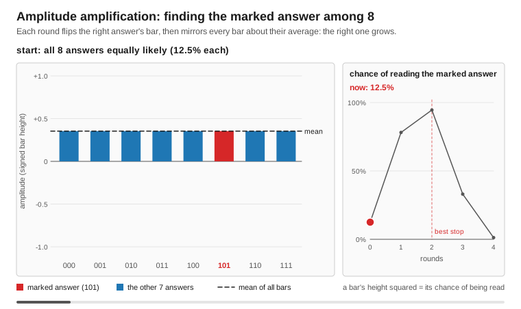
Amplitude amplification extends Grover's algorithm to work with arbitrary initial state preparations (not just uniform superposition). This enables quantum speedups for problems beyond simple database search.
Key Insight: Grover's algorithm is a special case where:
- Initial state = uniform superposition H^⊗n|0⟩
- Reflection operator = Grover diffusion operator
Amplitude amplification allows:
- Custom initial state preparation A|0⟩
- Reflection about A|0⟩ (automatically generated)
Example (▶ runnable: examples/Algorithms/AmplitudeAmplification.fsx):
open FSharp.Azure.Quantum
open FSharp.Azure.Quantum.GroverSearch
open FSharp.Azure.Quantum.Backends
open FSharp.Azure.Quantum.Core.BackendAbstraction

// Any IQuantumBackend — local simulator here, or a cloud backend for hardware.
let backend = LocalBackend.LocalBackend() :> IQuantumBackend

// State preparation A = H^⊗n (uniform superposition) as a gate circuit.
let prep =
    [ 0 .. 2 ] |> List.map CircuitBuilder.H
    |> List.fold (fun c g -> CircuitBuilder.addGate g c) (CircuitBuilder.empty 3)

match Oracle.forValue 5 3 with              // mark the basis state |101⟩ (value 5)
| Error e -> eprintfn "%s" e.Message
| Ok oracle ->
    let intent : AmplitudeAmplification.Unified.AmplitudeAmplificationIntent =
        { NumQubits = 3
          StatePreparation = prep
          Oracle = oracle
          Iterations = AmplitudeAmplification.optimalIterations 8 1 (1.0 / 8.0)
          Exactness = AmplitudeAmplification.Unified.Exact }

    match AmplitudeAmplification.Unified.execute backend intent with   // Result<QuantumState, _>
    | Ok finalState ->
        UnifiedBackend.measureState finalState 1000
        |> Array.countBy (fun bits -> bits |> Array.map string |> String.concat "")
        |> Array.iter (fun (state, count) -> printfn "  |%s⟩: %d counts" state count)
    | Error e -> eprintfn "Execution failed: %s" e.Message
Features:
- Custom state preparation (W-states, partial superpositions, arbitrary states)
- Runs on any gate-based
IQuantumBackend(LocalBackend, IonQ, Rigetti, ...): a cloud backend gets A and every iteration (oracle, then reflection) as one whole-circuit job - Automatic reflection operator generation (circuit-based A†)
- Grover equivalence verification (shows Grover as special case)
- Optimal iteration calculation for arbitrary initial success probability
- Measurement-based results (histogram of basis states)
Backend Limitations:
- Cloud backends return a state rebuilt from the measurement histogram (no amplitudes or phases) that carries the job's recorded counts;
UnifiedBackend.measureStateon it returns the job's own shots, never more than it measured (so the array can be shorter than requested), andPrimitives.samplereturns the job's counts - Suitable for algorithms that measure amplification results
- For amplitude/phase analysis, use local simulation
Use Cases:
- Quantum walk algorithms with non-uniform initial distributions
- Fixed-point search (where initial state biases toward solutions)
- Quantum sampling with amplification
- Fixed-amplitude search (building block for quantum counting)
Location: Algorithms/AmplitudeAmplification.fs (AmplitudeAmplification.Unified.execute)
Status: Well-tested and documented
Quantum Fourier Transform (QFT)
Quantum analog of the discrete Fourier transform - foundational building block for many quantum algorithms.
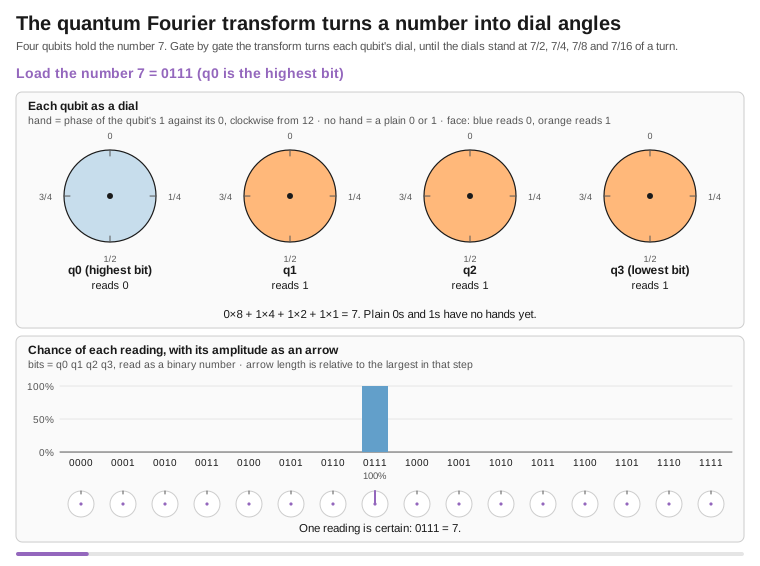
The QFT transforms computational basis states into the frequency basis with exponential speedup over the classical FFT. On n qubits (N = 2^n amplitudes):
- Classical FFT: O(n·2^n) operations on the amplitude vector
- Quantum QFT: O(n²) quantum gates (the amplitudes are not readable directly; they are sampled by measurement)
Mathematical Transform:
QFT: |j⟩ → (1/√N) Σₖ e^(2πijk/N) |k⟩
Example (▶ runnable: examples/Algorithms/QuantumFourierTransform.fsx):
open FSharp.Azure.Quantum.Algorithms
open FSharp.Azure.Quantum.Backends
open FSharp.Azure.Quantum.Core.BackendAbstraction

// Any IQuantumBackend — local simulator here, or a cloud backend for hardware.
let backend = LocalBackend.LocalBackend() :> IQuantumBackend

// Forward QFT on |0…0⟩ (5 qubits). QFT.defaultConfig = { ApplySwaps = true; Inverse = false; Shots = 1000 }.
match QFT.execute 5 backend QFT.defaultConfig with
| Ok result ->
    printfn "QFT applied: %d gates" result.GateCount           // result.FinalState : QuantumState
    UnifiedBackend.measureState result.FinalState 1000
    |> Array.countBy (fun bits -> bits |> Array.map string |> String.concat "")
    |> Array.iter (fun (state, count) -> printfn "  |%s⟩: %d counts" state count)
| Error e -> eprintfn "QFT failed: %s" e.Message

// Variants:
//   QFT.executeInverse 5 backend                                   // inverse QFT (QFT†)
//   QFT.executeNoSwaps 5 backend                                   // omit bit-reversal SWAPs (for QPE)
//   QFT.executeOnState state backend { QFT.defaultConfig with Inverse = true }   // apply to an existing state
Features:
- O(n²) gate complexity (exponential speedup over the classical O(n·2^n) FFT)
- Runs on any gate-based
IQuantumBackend(LocalBackend, IonQ, Rigetti, ...): a cloud backend gets the complete QFT circuit as one job, from |0…0⟩ or, withQFT.transformBasisState, from a basis state prepared in the same circuit.executeOnStatewith any other prepared state needs a simulator and is anErroron cloud - Controlled phase gates (CP) with correct decomposition
- Bit-reversal SWAP gates (optional for QPE)
- Inverse QFT (QFT†) for result decoding
- Angle validation (prevents NaN/infinity)
- Measurement-based results (histogram of basis states)
Backend Limitations:
- Cloud backends return a state rebuilt from the measurement histogram (no amplitudes or phases) that carries the job's recorded counts;
UnifiedBackend.measureStateon it returns the job's own shots, never more than it measured (so the array can be shorter than requested), andPrimitives.samplereturns the job's counts - Suitable for algorithms that measure QFT output (Shor's, Phase Estimation)
- For amplitude/phase analysis, use local simulation
Use Cases:
- Shor's Algorithm: Integer factorization (period finding step)
- Quantum Phase Estimation: Eigenvalue estimation for VQE improvements
- Period Finding: Hidden subgroup problems
- Quantum Signal Processing: Frequency domain analysis
Gate counts (QFT.estimateGateCount: n H + n(n-1)/2 controlled phases + ⌊n/2⌋ SWAPs):
- 3 qubits: 7 gates (3 H + 3 CPhase + 1 SWAP)
- 5 qubits: 17 gates (5 H + 10 CPhase + 2 SWAP)
- 10 qubits: 60 gates (10 H + 45 CPhase + 5 SWAP)
Location: Algorithms/QFT.fs (QFT.execute / executeOnState / executeInverse / executeNoSwaps)
Status: Well-tested and documented
Phase 2 Builders: QFT-Based Quantum Applications
High-level builders for cryptography, quantum chemistry, and research applications.
The library provides three advanced builders that wrap QFT-based quantum algorithms for real-world business scenarios:
Quantum Arithmetic Builder
Use Case: Cryptographic operations, RSA encryption, modular arithmetic
open FSharp.Azure.Quantum.QuantumArithmeticOps

// RSA encryption: m^e mod n
// The builder validates and returns a Result; bind it into execute
let encrypted =
    quantumArithmetic {
        operands 5 3           // message=5, exponent=3
        operation ModularExponentiate
        modulus 33             // RSA modulus
        qubits 6               // register; the circuit takes 2·6 + 5 = 17 qubits
    }
    |> Result.bind execute

match encrypted with
| Ok result ->
    printfn "Encrypted: %d" result.Value
    printfn "Gates: %d, Depth: %d" result.GateCount result.CircuitDepth
| Error err ->
    printfn "Error: %s" err.Message
C# API:
using static FSharp.Azure.Quantum.CSharpBuilders;

var encrypt = ModularExponentiate(baseValue: 5, exponent: 3, modulus: 33);
var result = ExecuteArithmetic(encrypt);
Business Applications:
- Cryptographic algorithm prototyping
- Educational RSA demonstrations
- Quantum arithmetic research
Example: examples/QuantumArithmetic/
Cryptographic Analysis Builder (Shor's Algorithm)
Use Case: RSA security assessment, post-quantum cryptography planning
open FSharp.Azure.Quantum.QuantumPeriodFinder

// Factor RSA modulus (security analysis)
// The builder validates and returns a Result; bind it into solve
let factorResult =
    periodFinder {
        number 15              // Composite to factor
        precision 8            // QPE precision
        maxAttempts 10         // Retries (probabilistic)
    }
    |> Result.bind solve

match factorResult with
| Ok result ->
    match result.Factors, result.FactorSource with
    | Some (p, q), FSharp.Azure.Quantum.Algorithms.ShorsTypes.FactorSource.QuantumPeriodFinding ->
        printfn "Factors: %d × %d (period %d measured by quantum period finding)" p q result.Period
    | Some (p, q), _ ->
        // N was even, or the drawn base shared a factor with N: no circuit ran
        printfn "Factors: %d × %d (classical preprocessing)" p q
    | None, _ ->
        printfn "Try again (probabilistic)"
| Error err ->
    printfn "Error: %s" err.Message
FactorSource says where the factors came from, so a lucky gcd is never reported as a quantum result. The period finding runs gate by gate on the local simulator, as one native intent on the topological backend, and as one whole-circuit job per base tried on a cloud backend. Even N = 15 is a deep circuit, far beyond what today's hardware runs without errors.
C# API:
var problem = FactorInteger(15, precision: 8);
var result = ExecutePeriodFinder(problem);
Business Applications:
- Security consulting (quantum threat assessment)
- Post-quantum cryptography migration planning
- Cryptanalysis research and education
Example: examples/CryptographicAnalysis/
Phase Estimation Builder (Quantum Chemistry)
Use Case: Drug discovery, molecular simulation, materials science
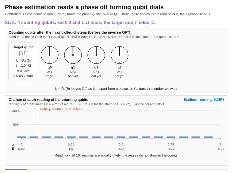
open System
open FSharp.Azure.Quantum.QuantumPhaseEstimator
open FSharp.Azure.Quantum.Algorithms.QPE

// Estimate the eigenphase of a unitary (the core step of QPE-based energy estimation)
// The builder validates and returns a Result; bind it into estimate
let energyResult =
    phaseEstimator {
        unitary (RotationZ (Math.PI / 3.0))  // Unitary operator U
        precision 12                          // 12-bit phase precision
    }
    |> Result.bind estimate

match energyResult with
| Ok result ->
    printfn "Phase: %.6f" result.Phase
    printfn "Eigenphase angle: %.4f rad" (result.Phase * 2.0 * Math.PI)
| Error err ->
    printfn "Error: %s" err.Message
C# API:
var problem = EstimateRotationZ(Math.PI / 3.0, precision: 12);
var result = ExecutePhaseEstimator(problem);
Business Applications:
- Pharmaceutical drug discovery (binding energy)
- Materials science (electronic properties)
- Quantum chemistry simulations
Example: examples/PhaseEstimation/
Phase 2 Builder Features:
- Business-focused APIs hiding quantum complexity
- F# computation expressions + C# fluent API
- Comprehensive examples with real-world scenarios
- Educational value for quantum algorithm learning
- Run on the local simulator or, as whole-circuit jobs, on the gate-based cloud backends
- NISQ limitations: Toy examples only (about 20 qubits)
- Requires fault-tolerant quantum computers for production use (e.g. RSA key lengths)
Current Status: Educational/research focus - Demonstrates quantum algorithms, but current hardware is insufficient for real-world applications
| Feature Category | FSharp.Azure.Quantum | IBM Qiskit | Microsoft Azure Quantum SDK | Google Cirq | Amazon Braket SDK |
|---|---|---|---|---|---|
| Primary Language | F# (with C# interop) | Python | Python, C#, Q# | Python | Python |
| License | Unlicense (Public Domain) | Apache 2.0 | MIT | Apache 2.0 | Apache 2.0 |
| Target Audience | .NET developers, optimization problems | General quantum computing | Enterprise quantum developers | Google hardware users | AWS cloud users |
| 🎯 OPTIMIZATION SOLVERS | |||||
| MaxCut | ✅ Built-in (QAOA) | ✅ Qiskit Optimization | ❌ Manual | ❌ Manual | ❌ Manual |
| Knapsack | ✅ Built-in (QAOA) | ✅ Qiskit Optimization | ❌ Manual | ❌ Manual | ❌ Manual |
| TSP | ✅ Built-in (QAOA) | ✅ Qiskit Optimization | ❌ Manual | ❌ Manual | ❌ Manual |
| Portfolio Optimization | ✅ Built-in (QAOA) | ✅ Qiskit Finance | ❌ Manual | ❌ Manual | ❌ Manual |
| Task Scheduling | ✅ Built-in (QAOA) | ❌ Manual | ❌ Manual | ❌ Manual | ❌ Manual |
| Network Flow | ✅ Built-in (QAOA) | ❌ Manual | ❌ Manual | ❌ Manual | ❌ Manual |
| Graph Coloring | ✅ Built-in (QAOA) | ❌ Manual implementation | ❌ Manual | ❌ Manual | ❌ Manual |
| 🤖 QUANTUM MACHINE LEARNING | |||||
| VQC (Variational Classifier) | ✅ Built-in | ✅ Qiskit Machine Learning | ❌ Manual | ✅ TFQ integration | ✅ Built-in |
| Quantum Kernel SVM | ✅ Built-in | ✅ Qiskit Machine Learning | ❌ Manual | ❌ Limited | ✅ Built-in |
| Feature Maps | ✅ ZZ, Pauli, Angle | ✅ Extensive library | ❌ Manual | ✅ Via TFQ | ✅ Built-in |
| Variational Forms | ✅ RealAmplitudes, EfficientSU2 | ✅ Extensive ansatz library | ❌ Manual | ✅ Via Cirq | ✅ Built-in |
| AutoML Integration | ✅ Built-in | ❌ External tools | ❌ No | ❌ No | ❌ No |
| 📊 BUSINESS PROBLEM BUILDERS | |||||
| Anomaly Detection | ✅ Built-in | ❌ Manual | ❌ No | ❌ No | ❌ No |
| Binary Classification | ✅ Built-in | ✅ Qiskit ML | ❌ No | ❌ No | ❌ No |
| Predictive Modeling | ✅ Built-in | ❌ Manual | ❌ No | ❌ No | ❌ No |
| Similarity Search | ✅ Built-in | ❌ Manual | ❌ No | ❌ No | ❌ No |
| 🔬 QUANTUM ALGORITHMS | |||||
| QAOA | ✅ Production-ready, auto-optimized (Nelder-Mead) | ✅ Qiskit Optimization | ✅ Q# samples | ✅ Manual | ✅ Built-in |
| VQE | ✅ Built-in (chemistry) | ✅ Qiskit Nature | ✅ Q# samples | ✅ Built-in | ✅ Built-in |
| Grover's Algorithm | ✅ Educational | ✅ Built-in | ✅ Q# samples | ✅ Built-in | ✅ Built-in |
| Shor's Algorithm | ✅ Educational (period finder) | ✅ Built-in | ✅ Q# samples | ✅ Built-in | ✅ Built-in |
| QFT | ✅ Built-in | ✅ Built-in | ✅ Q# built-in | ✅ Built-in | ✅ Built-in |
| HHL (Linear Systems) | ✅ Built-in | ✅ Qiskit Aqua | ❌ Manual | ❌ Manual | ❌ Manual |
| Amplitude Amplification | ✅ Built-in | ✅ Built-in | ✅ Q# built-in | ✅ Built-in | ❌ Manual |
| 🖥️ LOCAL SIMULATION | |||||
| Local Simulator | ✅ Built-in (memory-derived, ≤30) | ✅ Aer (≤30 qubits) | ✅ Full-state (≤30 qubits) | ✅ Built-in (≤20 qubits) | ✅ Local simulator |
| Noise Simulation | ✅ Density matrix (NoisyLocalBackend, ≤ 8 qubits) |
✅ AerSimulator noise models | ✅ Open/Closed systems | ✅ Built-in | ✅ Built-in |
| GPU Acceleration | ⚠️ Via CUDA-Q source hand-off (CudaQBridge) |
✅ Aer GPU | ✅ Yes | ✅ Yes | ✅ Yes |
| State Vector | ✅ Pure F# implementation | ✅ C++ backend | ✅ C++ backend | ✅ C++ backend | ✅ C++ backend |
| ☁️ CLOUD BACKENDS | |||||
| Azure Quantum (IonQ) | ✅ Native | ✅ Via Qiskit Runtime | ✅ Native | ❌ No | ❌ No |
| Azure Quantum (Rigetti) | ✅ Native | ✅ Via Qiskit Runtime | ✅ Native | ❌ No | ❌ No |
| IBM Quantum | ❌ Via OpenQASM export | ✅ Native | ❌ No | ❌ No | ❌ No |
| D-Wave Quantum Annealer | ✅ Native | ✅ Via Ocean SDK | ✅ Native | ❌ No | ✅ Native |
| AWS Braket | ✅ Via FSharp.Azure.Quantum.Braket plugin |
✅ Via plugin | ❌ No | ❌ No | ✅ Native |
| Google Quantum | ❌ Via OpenQASM export | ✅ Via plugin | ❌ No | ✅ Native | ❌ No |
| 🔄 INTEROPERABILITY | |||||
| OpenQASM 2.0 Import | ✅ Full support | ✅ Native | ✅ Via conversion | ✅ Full support | ✅ Full support |
| OpenQASM 2.0 Export | ✅ Full support | ✅ Native | ✅ Via conversion | ✅ Full support | ✅ Full support |
| QUIL | ✅ Export (Rigetti backend) | ❌ Via plugin | ✅ Rigetti native | ❌ No | ✅ Rigetti support |
| 🛡️ ERROR MITIGATION | |||||
| Zero-Noise Extrapolation | ✅ Built-in (typically 30-50% reduction) | ✅ Qiskit Experiments | ❌ Manual | ✅ Via Mitiq integration | ❌ Manual |
| Probabilistic Error Cancellation | ✅ Built-in (typically 50-80% reduction) | ✅ Via Mitiq | ❌ Manual | ✅ Via Mitiq integration | ❌ Manual |
| Readout Error Mitigation | ✅ Built-in (typically 50-90% reduction) | ✅ Qiskit Experiments | ❌ Manual | ✅ Via Mitiq integration | ❌ Manual |
| Automatic Strategy Selection | ✅ Built-in | ❌ Manual | ❌ No | ❌ Manual | ❌ No |
| 💻 API DESIGN | |||||
| Computation Expressions | ✅ F# native pattern | ❌ N/A (Python) | ❌ No | ❌ N/A (Python) | ❌ N/A (Python) |
| Type Safety | ✅ F# compile-time checks | ⚠️ Python dynamic typing | ⚠️ Python/C# mixed | ⚠️ Python dynamic typing | ⚠️ Python dynamic typing |
| Fluent API (C#) | ✅ Built-in | ❌ N/A | ✅ Native C# | ❌ N/A | ❌ N/A |
| Functional Programming | ✅ F# first-class | ❌ Object-oriented | ⚠️ Mixed | ⚠️ Mixed | ❌ Object-oriented |
| Result Type Error Handling | ✅ F# Result<T,E> | ❌ Exceptions | ❌ Exceptions | ❌ Exceptions | ❌ Exceptions |
| 🤖 HYBRID CLASSICAL-QUANTUM | |||||
| Automatic Problem Routing | ✅ HybridSolver (optional) | ❌ Manual | ❌ Manual | ❌ Manual | ❌ Manual |
| Classical Fallback | ✅ Built-in via HybridSolver (small problems, below 50 variables; opt-in) | ❌ Manual | ❌ No | ❌ No | ❌ No |
| Cost Guards | ✅ HybridSolver budget limits (CostEstimation), JobBudget job caps on cloud backends |
❌ Manual | ❌ Manual | ❌ Manual | ❌ Manual |
| Quantum Advantage Analysis | ✅ Built-in reasoning (QuantumAdvisor) | ❌ Manual | ❌ No | ❌ No | ❌ No |
| 🧪 QUANTUM CHEMISTRY | |||||
| VQE for Molecules | ✅ Built-in (H₂, H₂O) | ✅ Qiskit Nature | ✅ Q# Chemistry | ✅ OpenFermion integration | ✅ Built-in |
| Hamiltonian Construction | ✅ Built-in | ✅ Qiskit Nature | ✅ Broombridge format | ✅ OpenFermion | ✅ OpenFermion |
| UCC Ansatz | ✅ Built-in | ✅ Qiskit Nature | ✅ Q# Chemistry | ✅ OpenFermion | ✅ Built-in |
| 📚 ECOSYSTEM | |||||
| Circuit Visualization | ❌ Mermaid, or Export to OpenQASM → Qiskit | ✅ Native (matplotlib) | ✅ Q# visualizer | ✅ Native (matplotlib) | ✅ Native (matplotlib) |
| Documentation Quality | ✅ Comprehensive (MD docs) | ✅ Tutorials | ✅ Microsoft Docs | ✅ Google Docs | ✅ AWS Docs |
| Example Projects | ✅ 30+ working examples | ✅ Tutorials | ✅ Samples | ✅ Tutorials | ✅ Examples |
| Community Size | ⚠️ Small (new library) | ✅ Large | ⚠️ Medium | ✅ Medium | ⚠️ Medium |
| 🔧 DEVELOPMENT EXPERIENCE | |||||
| IDE Support | ✅ Visual Studio, VS Code | ✅ Jupyter, VS Code | ✅ Visual Studio, VS Code | ✅ Jupyter, VS Code | ✅ Jupyter, VS Code |
| REPL/Interactive | ✅ F# Interactive (FSI) | ✅ Jupyter Notebooks | ✅ Q# Jupyter | ✅ Jupyter Notebooks | ✅ Jupyter Notebooks |
| Package Manager | ✅ NuGet | ✅ pip | ✅ NuGet, pip | ✅ pip | ✅ pip |
| Installation | ✅ dotnet add package | ✅ pip install qiskit | ✅ pip install azure-quantum | ✅ pip install cirq | ✅ pip install amazon-braket-sdk |
| 💰 COST | |||||
| Local Development | ✅ Free | ✅ Free | ✅ Free | ✅ Free | ✅ Free |
| Cloud QPU Access | 💰 Azure Quantum pricing | 💰 IBM Quantum pricing | 💰 Azure Quantum pricing | 💰 Google Quantum pricing | 💰 AWS Braket pricing |
| D-Wave Quantum | 💰 D-Wave Leap pricing | 💰 Via Ocean SDK | 💰 Azure marketplace | ❌ N/A | 💰 AWS Braket |
Topological Quantum Computing
Simulate topological quantum computers using anyon braiding - the approach behind Microsoft's Majorana quantum computing program.
Unlike gate-based quantum computing (which uses qubits and gates), topological quantum computing encodes information in anyons (exotic quasiparticles) and performs operations by braiding their worldlines. This provides inherent fault-tolerance through topological protection.
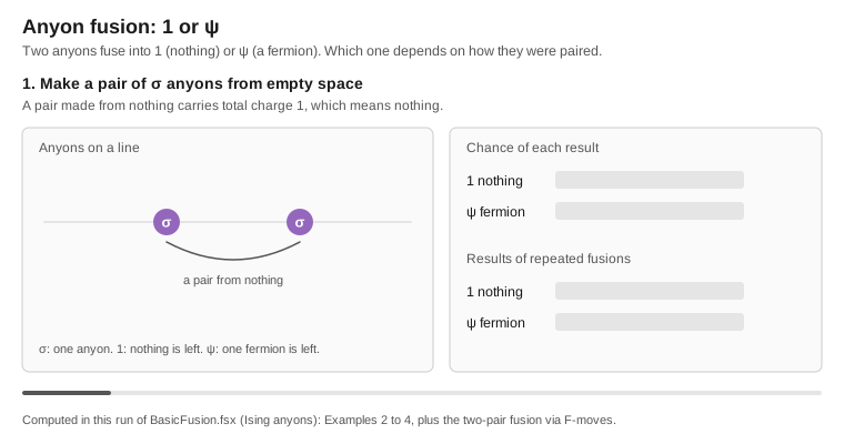
Quick Example: Ising Anyons (Microsoft Majorana)
open FSharp.Azure.Quantum.Topological

// Create backend for Ising anyons (Microsoft's approach), up to 10 anyons
let backend = TopologicalUnifiedBackendFactory.createIsing 10

// Create entangled state via braiding
let program = topological backend {
    // Initialize 2 logical qubits (6 sigma anyons)
    do! TopologicalBuilder.initialize AnyonSpecies.AnyonType.Ising 2

    // Braiding creates entanglement geometrically
    do! TopologicalBuilder.braid 0  // Braid anyons 0-1
    do! TopologicalBuilder.braid 2  // Braid anyons 2-3
    do! TopologicalBuilder.braid 1  // Braid anyons 1-2 (entangles the qubits)

    // Measure fusion outcome
    let! outcome = TopologicalBuilder.measure 0
    return outcome
}

task {
    match! TopologicalBuilder.execute backend program with
    | Ok particle ->
        printfn "Fusion outcome: %A" particle  // Vacuum or Psi
    | Error err ->
        printfn "Error: %s" err.Message
}
Key Concepts
Anyons:
- Ising anyons:
{1 (vacuum), σ (sigma), ψ (psi)}- Microsoft's Majorana approach - Fibonacci anyons:
{1, τ}- Theoretical universal braiding - Fusion rule for Ising:
σ × σ = 1 + ψ(creates quantum superposition)
Operations:
- Braiding: Exchange anyons (replaces quantum gates)
- Fusion: Measurement (collapses superposition to classical outcome)
- F-moves: Change fusion tree basis (advanced)
- Error Correction: Toric code (MWPM), surface codes (planar, color), anyonic charge correction
Why topological qubits are studied:
- Topological protection: information is stored non-locally, so local noise does not change it
- Passive error suppression: errors need a non-local process to affect the encoded state
- This is a simulator; topological hardware is still experimental
Comparison: Gate-Based vs Topological
| Aspect | Gate-Based QC | Topological QC |
|---|---|---|
| State | Qubit amplitudes | Fusion trees |
| Operations | H, CNOT, RZ gates | Braid, Measure |
| Error Correction | Active (surface codes) | Passive (topology) |
| Hardware | IonQ, Rigetti, IBM | Microsoft Majorana (experimental) |
Examples
See examples/Topological/ for complete examples:
- BasicFusion.fsx - Fusion rules and statistics
- BellState.fsx - Creating entanglement via braiding
- BackendComparison.fsx - Ising vs Fibonacci anyons
Documentation
- Getting Started:
docs/topological/getting-started.md(install, build, first computation) - Documentation Index:
docs/topological/index.md(full guide with learning paths) - Library README:
src/FSharp.Azure.Quantum.Topological/README.md - Examples:
examples/Topological/(10 runnable.fsxscripts) - Format Spec:
docs/topological-format-spec.md(import/export)
Neutral-Atom (Rydberg) Analog Mode
A third machine paradigm alongside gate and topological: neutral-atom devices are programmed as an analog time evolution rather than a gate circuit. You place atoms at positions and drive them with a global pulse (Rabi frequency Ω, detuning Δ); the van-der-Waals interaction produces the Rydberg blockade (nearby atoms can't both be excited), which makes these machines natively good at Maximum Independent Set.
Algorithms.NeutralAtom fits this into the unified model the same way BraidToGate fits
topological braids — it Trotterizes the analog Hamiltonian into a gate circuit (drive →
RX, detuning → P, interaction → CP), so a Rydberg program runs on any IQuantumBackend.
open FSharp.Azure.Quantum.Core.BackendAbstraction
open FSharp.Azure.Quantum.Backends
open FSharp.Azure.Quantum.Algorithms
open FSharp.Azure.Quantum.Algorithms.NeutralAtom

let backend = LocalBackend.LocalBackend() :> IQuantumBackend
// 3-atom path A–B–C; neighbours blockade, so the max independent set is {A, C} = "101".
let register = [ { X = 0.0; Y = 0.0 }; { X = 1.0; Y = 0.0 }; { X = 2.0; Y = 0.0 } ]
let program = maximumIndependentSetProgram register 30.0 1.0 3.0 12.0   // adiabatic detuning sweep
NeutralAtom.simulate backend program 120 4000   // Result<Map<string,int>> — peaks on "101"
Small registers only (it Trotterizes onto the state-vector simulator). ▶ Runnable example:
examples/NeutralAtom/RydbergMaxIndependentSet.fsx
Run on real neutral-atom hardware — Pasqal. The same RydbergProgram can be submitted
natively to Pasqal on Azure Quantum: Algorithms.Pasqal compiles it to a Pulser
abstract-representation sequence (Pasqal.toPulserJson) and submits it to a Pasqal target
(Pasqal.submitAndWaitForResultsAsync httpClient workspaceUrl program shots "pasqal.qpu.fresnel" cancellationToken).
So one analog program has three execution paths — Trotterized onto any gate backend for local
simulation, native analog execution on Pasqal (Azure Quantum, via Pulser), or native analog
execution on QuEra Aquila (AWS Braket, via QuEra.toAhsProgram → a braket.ir.ahs.program
AHS sequence; QuEra.parseAhsResult reads the results back).
AWS Braket — a separate plugin (FSharp.Azure.Quantum.Braket)
The core package stays Azure-first and AWS-SDK-free: it only produces the formats Braket
consumes — OpenQASM 3.0 for gate devices (OpenQasm.exportV3) and AHS for QuEra
(QuEra.toAhsProgram), both pure and testable. The actual submission lives in a separate
FSharp.Azure.Quantum.Braket package (the only one that references AWSSDK.Braket):
BraketExecution.BraketBackend— a gateIQuantumBackendthat submits OpenQASM 3.0 to any Braket gate device by ARN: IonQ, Rigetti, IQM, OQC, Infleqtion, and the SV1/DM1/TN1 simulators (Braket.Devices.*). Results come back as aQuantumStatereconstructed from the measurement histogram (dense up toStateVector.maxQubits, sparse through 31,MeasurementHistogramabove — no width limit);ExecuteToHistogramAsyncreturns the raw bitstring→count histogram at any width.BraketExecution.submitAhsAsync— submits a neutral-atomRydbergProgramto QuEra Aquila.
So adding the AWS SDK is opt-in (reference the plugin); users who only need Azure never pull it in.
NeutralAtom.solveMaximumIndependentSet runs the whole thing end-to-end and returns the best
independent set as atom indices. Beyond optimisation, the module also does analog quantum
simulation: NeutralAtom.quench builds a sudden constant-drive pulse, NeutralAtom.evolve
returns the final state, and NeutralAtom.rydbergDensities reads each atom's occupation ⟨nᵢ⟩ —
so you can watch Rabi and blockade dynamics (a single atom traces ⟨n⟩ = sin²(Ωt/2); a blockaded
pair's total excitation is capped). NeutralAtom.optimizeAnalog closes the loop with
variational pulse shaping (analog QAOA): tune pulse knobs to minimise ⟨H⟩, reusing the
shared optimiser — the analog counterpart of variational gate optimisation.
Annealing is a first-class path too
Because D-Wave backends implement IQuantumBackend (they reverse-extract the QUBO from the
circuit and anneal it), a QUBO problem targets annealing hardware through the same unified
API — just pass a D-Wave backend:
open System.Threading
open FSharp.Azure.Quantum
open FSharp.Azure.Quantum.Core.BackendAbstraction
open FSharp.Azure.Quantum.Backends.DWaveBackend
open FSharp.Azure.Quantum.Backends.DWaveTypes

let triangle = MaxCut.createProblem ["A"; "B"; "C"] [("A", "B", 1.0); ("B", "C", 1.0); ("C", "A", 1.0)]
let annealer = MockDWaveBackend(Advantage_System6_1, seed = 42) :> IQuantumBackend
MaxCut.solveAsync triangle (Some annealer) CancellationToken.None   // solved by simulated/real annealing, not QAOA gates
Contributing
Contributions welcome!
Development principles:
- Keep solvers quantum-first (no silent classical fallback; classical code only as baselines or through
HybridSolver) - Follow F# coding conventions
- Provide C# interop for new builders
- Include comprehensive tests
- Document QAOA encodings for new problem types
License
Unlicense - Public domain. Use freely for any purpose.
Support
- Documentation: docs/
- Issues: GitHub Issues
- Examples: examples/
Status: Quantum-first architecture, 7 problem builders, full QAOA implementation
| Product | Versions Compatible and additional computed target framework versions. |
|---|---|
| .NET | net10.0 is compatible. net10.0-android was computed. net10.0-browser was computed. net10.0-ios was computed. net10.0-maccatalyst was computed. net10.0-macos was computed. net10.0-tvos was computed. net10.0-windows was computed. |
-
net10.0
- Azure.Identity (>= 1.21.0)
- FSharp.Core (>= 10.1.302)
- MathNet.Numerics (>= 5.0.0)
- MathNet.Numerics.FSharp (>= 5.0.0)
- Microsoft.Extensions.Logging (>= 10.0.12)
- OpenTelemetry (>= 1.19.1)
- OpenTelemetry.Exporter.Console (>= 1.19.1)
- OpenTelemetry.Instrumentation.Http (>= 1.19.0)
- Serilog (>= 4.4.0)
- Serilog.Sinks.Console (>= 6.1.1)
- Serilog.Sinks.File (>= 7.0.0)
NuGet packages (2)
Showing the top 2 NuGet packages that depend on FSharp.Azure.Quantum:
| Package | Downloads |
|---|---|
|
FSharp.Azure.Quantum.Topological
Topological quantum computing plugin for FSharp.Azure.Quantum. Provides anyon theory (Ising/Fibonacci/SU(2)_k), braiding compilation, gate-to-braid conversion, Majorana (tetron) hardware device profiles and noise models, and topological file format (.tqp). Includes Majorana 1 (Al–InAs) and Majorana 2 (InAs–Pb) hardware profiles. Seamlessly integrates with main package algorithms (Grover, QFT, QAOA) via IQuantumBackend interface. Requires FSharp.Azure.Quantum v1.3.10+. |
|
|
FSharp.Azure.Quantum.Braket
AWS Braket plugin for FSharp.Azure.Quantum. Submits circuits to Braket gate QPUs (IonQ, Rigetti, IQM, OQC, Infleqtion) and simulators (SV1/DM1/TN1) via OpenQASM 3.0, and neutral-atom analog programs to QuEra Aquila via the Braket AHS format. This is the only package that depends on the AWS SDK — the core FSharp.Azure.Quantum package stays AWS-free. Requires FSharp.Azure.Quantum. |
GitHub repositories
This package is not used by any popular GitHub repositories.
| Version | Downloads | Last Updated |
|---|---|---|
| 1.6.2 | 107 | 10/10/2026 |
| 1.6.1 | 103 | 10/9/2026 |
| 1.6.0 | 99 | 10/9/2026 |
| 1.5.2 | 121 | 10/2/2026 |
| 1.5.1 | 105 | 10/1/2026 |
| 1.5.0 | 111 | 10/1/2026 |
| 1.4.15 | 118 | 9/30/2026 |
| 1.4.12 | 111 | 9/29/2026 |
| 1.4.11 | 124 | 9/26/2026 |
| 1.4.9 | 133 | 9/20/2026 |
| 1.4.8 | 120 | 9/18/2026 |
| 1.4.7 | 155 | 8/1/2026 |
| 1.4.6 | 162 | 7/11/2026 |
| 1.4.5 | 149 | 7/6/2026 |
| 1.4.4 | 155 | 7/3/2026 |
| 1.4.3 | 156 | 7/1/2026 |
| 1.4.2 | 161 | 6/30/2026 |
| 1.4.1 | 155 | 6/12/2026 |
| 1.3.12 | 163 | 4/1/2026 |
| 1.3.11 | 166 | 3/31/2026 |
v1.6.2: Neighbourhood search for QUBOs that no exact split cuts; drone examples at swarm scale and on a map
- ADDED (QuboSplitting): searchNeighbourhoodsAsync improves any problem one block at a time with the rest fixed (Neighbourhoods: blocks per sweep, a block's QUBO, Apply, Score, Accept); runs are blocks times sweeps; quboNeighbourhoods and searchQuboNeighbourhoodsAsync for a dense QUBO
- ADDED (QaoaExecutionHelpers): SplitSettings.MaxSweeps (default 0, off) lets runQaoaAsync search a QUBO that neither cuts nor fits; SplitReport.Sweeps tells a heuristic answer from an exact join
- EXAMPLES (SwarmChoreography): a swarm wider than one circuit is assigned in blocks of ⌊√limit⌋ drones (BlockAssignment); --drones n scale run, --lights light show, show.svg with the drones' light colours
- EXAMPLES (FireAirBridge): --fire and --water name the scenario as points; --map draws the run on OpenStreetMap tiles with the round's candidate corridors, the plan, the fire and the decisions, zoomable
v1.6.1: Grover lowers an oracle once per search; resource estimates no longer judge by a fixed qubit count
- CHANGED (Grover): a predicate oracle is lowered to gates once per search, not once per iteration count tried and again for a cloud backend's whole-circuit job
- CHANGED: the period finder and phase estimator builders' estimateResources judge feasibility by QPE.MaxCountingQubits and MaxPrecision, not a fixed 20 qubits
v1.6.0: qubit limits come from the backend; QUBO splitting joins by variable elimination within a run budget
- BREAKING: Types.NisqPracticalQubits and the fixed qubit caps are removed; every width check uses UnifiedBackend.getRunnableQubits (local simulator: 20 by default, FSAQ_MAX_CIRCUIT_QUBITS), and a backend with no declared limit is not refused
- BREAKING: SplitSettings.MaxFixedVariables removed; MaxShareRuns bounds the circuit runs of either split, counted before any run (conditioning: 2^boundary per piece; shares: block runs)
- BREAKING: QuboSplitting.ConditioningLimits.MaxRuns replaces MaxFixedVariables; MostFixedVariables removed, MostJoinSpan (20) added
- CHANGED: conditioning joins its pieces by min-sum variable elimination (cost 2^join width, not 2^fixed variables) and fixes any number of variables; a split wider than MostJoinSpan is refused before any run
- CHANGED: QuboSplitting refuses a dense QUBO before the separator search (degeneracy of the variables the run budget forces to be fixed)
- CHANGED (Grover): Grover.search refuses an oracle wider than the backend runs, before any circuit; oracles index up to 30 qubits (Oracle.MaxIndexQubits; SAT, clique and colouring caps of 20, 10 vertices and 8 colours removed)
- ADDED: UnifiedBackend.requireRunnableQubits, runnableQubitsError and runnableQubitsReason (one width check and message for every algorithm and builder); LocalBackendFactory.orLocal
- CHANGED: Deutsch-Jozsa, Bernstein-Vazirani and Simon refuse only inputs wider than the backend runs (were 20, 20 and 2·10 qubits)
- CHANGED: tree search, constraint solver and pattern matcher builders check width against the backend in solve (were 16 qubits, depth 8, branching 256, 2^16 items); estimateResources no longer judges feasibility against 16 qubits
- CHANGED (chemistry): VQE and QPE refuse a Hamiltonian wider than the backend runs (was 20 qubits on every backend)
- BREAKING (chemistry): QPE.MaxTotalQubits removed; default counting qubits follow the backend (8 with no limit); DefaultCountingQubits, MinCountingQubits and MaxCountingQubits added
- CHANGED: linear system, period finder and phase estimator builders check circuit width against the backend (removed the 12 eigenvalue-qubit, 16×16, 20-qubit, N ≤ 10000, precision ≤ 20, target ≤ 10 and total ≤ 25 caps); phase estimator precision ≤ 30
- CHANGED (QPE, Shor): circuits are budgeted against the backend's runnable qubits, not the local simulator's; QPE counting qubits ≤ 30 (QPE.MaxCountingQubits); Shor accepts N ≤ 46340 (Shor.MaxNumberToFactor, int32 arithmetic; was 1000) and an explicit precision below the register width when it fits; a precision wider than the backend leaves room for is reduced, not refused
- CHANGED: the period finder builder sizes a native-QPE backend by counting and register qubits only (Shor.narrowestPeriodFindingQubits)
- CHANGED: QaoaSimulator runs up to StateVector.practicalCircuitQubits (was 16); CircuitValidator's local-simulator preset follows it (was 16)
- CHANGED (ML): binary classification (VQC and hybrid), predictive models and anomaly detection use one qubit per feature, refused only above the backend's runnable qubits (were 8, 5 and 8 features); anomaly detection reports its real NumQubits
- FIXED: VQC prediction refuses a sample whose width differs from the trained features (was silently truncated)
- CHANGED: ConstraintScheduler accepts more than 50 tasks and SocialNetworkAnalyzer more than 100 people; the SocialNetworkAnalyzer Grover path refuses a network wider than the backend runs
v1.5.2: BB84 and E91 draw their secrets from the OS cryptographic generator; BB84 checks its parameters
- CHANGED: BB84 and E91 without a seed draw bits, bases and the eavesdropping-check sample from the OS cryptographic generator (new Core.CryptographicRandom, a System.Random); BB84's check sample is a uniform shuffle, so a seeded run picks different positions than before
- CHANGED: BB84 returns a validation error for a sample ratio outside (0, 1) or too close to 1 for one run, for a check sample that comes out empty and for a key length below 1 (was a key reported secure with no check, or an exception)
v1.5.1: QUBO encoding fixes; QAOA solutions report how often they were sampled
- FIXED (network flow): the demand term is a squared penalty, so the QUBO minimum is the cheapest flow that serves every sink; solveWithShotsAsync and solveWithDefaultsAsync optimise the angles (2 layers); solveWithQaoaConfigAsync takes a QaoaSolverConfig
- FIXED (TSP): every step is charged in the direction taken, return leg included; the penalty scales with the distances; only a permutation matrix decodes to a tour (no padding), so few shots can end in a "no valid tour" error. 2 optimised layers by default (QuantumTspConfig.NumLayers, QuantumTspSolution.LayerParameters); a 4-city default solve takes minutes on the simulator
- FIXED (bin packing): capacity is an inequality with slack bits (4,3,3 into 6 takes 12 qubits, was 8); sizes are rescaled to integers; isValid is strict; repair always returns a valid packing; PackingResult gains WasRepaired and Sampling
- FIXED (binary ILP): the slack range covers negative coefficients; non-integer coefficients and bounds are rescaled or rejected; feasible negative bounds are accepted
- FIXED (knapsack): non-integer weights and capacities are rescaled or rejected; the subset-sum loop adds no exclusion term
- FIXED (portfolio): a holding limit below the asset count is a QUBO term with slack bits
- FIXED (ConstraintScheduler): resources with capacities get a QUBO with each capacity and the hard constraints; IsFeasible requires one resource per task, capacity, hard constraints and the budget
- FIXED (drug discovery): diverse selection rescales costs to integers; the influence penalty covers the synergy term; QAOA selection takes 1000 final shots (DrugDiscoveryConfiguration.SelectionShots)
- CHANGED (task scheduling): optimised angles (solveWithConfigAsync), samples decode strictly one-hot; Solution gains WasRepaired and Sampling
- CHANGED (clique): recombine keeps the heaviest clique, the measure the QUBO optimises
- BREAKING: Knapsack.findAllExactCombinationsAsync, findAllCapturedItemsAsync and findAllValidCombinationsAsync return Task<QuantumResult<…>>; a quantum error is returned instead of a classical answer
- FIXED (benchmarks): benchmarkClassicalTSPAsync and benchmarkClassicalPortfolioAsync time the classical solvers
- ADDED: every QAOA solver solution has Sampling: SampleStatistics option (Shots, Qubits, Hits, Valid; HitRate, ValidRate, UniformRate, ShotsFor confidence). Code that constructs a solution record adds `Sampling = None`
- ADDED: QaoaExecutionHelpers.runQaoaSampledAsync (every final sample, QaoaRun) and sampleStatistics; Qubo.squaredLinearPenalty, boundedSlackWeights, tryScaleToIntegers
- ADDED: QuboSplitting runs a problem wider than the backend as circuits that fit, trading qubits for runs. Conditioning fixes a few variables of a sparse QUBO (MaxCut, vertex cover, clique, matching, set cover, MAX-SAT, binary ILP, drug-discovery solvers); blocks cut a knapsack into pieces without slack bits (QuantumKnapsackSolver.solveInBlocksAsync, and solveAsync). A split solution reports Split: SplitReport (runs, widest piece, fixed variables, blocks) and has Sampling = None
- ADDED: QuantumKnapsackSolver.findAllExactCombinationsAsync leaves out items heavier than the target and splits a search over more items than the backend runs into halves joined over their partial sums (SubsetSumConfig.Splitting; SubsetSumResult.Split)
- ADDED: the Azure Quantum backends take maxQubits, which replaces the built-in qubit limit of the target (CloudBackendHelpers.qubitLimit); the built-in figures are defaults
- CHANGED: a Quantinuum target this version does not know reports no qubit limit (was 20)
- ADDED: SplitSettings (Splitting on QaoaSolverConfig and on the MaxCut, Knapsack and subset-sum configs): Policy Never | OnSimulators (default: backends that bill every circuit are never split unasked) | Always, MaxPieceQubits, MaxFixedVariables (8), MaxShareRuns (256), MaxBlockItems (12). A problem that cannot be split runs as one circuit while the backend holds it. Full literals of those config records add `Splitting = QaoaExecutionHelpers.defaultSplitSettings`